class: title-slide, middle <style type="text/css"> .title-slide { background-image: url('img/bg.jpg'); background-color: #23373B; background-size: contain; border: 0px; background-position: 600px 0; line-height: 1; } </style> # Lecture 1 <hr width="65%" align="left" size="0.3" color="orange"></hr> ## Introduction to scientific computing <hr width="65%" align="left" size="0.3" color="orange" style="margin-bottom:40px;"></hr> .instructors[ **Introduction to R for Biologists** - Lauren Talluto ] --- layout: true # Why scientific computing? --- - Growth in big data applications, remote sensing, monitoring, sequencing .image60[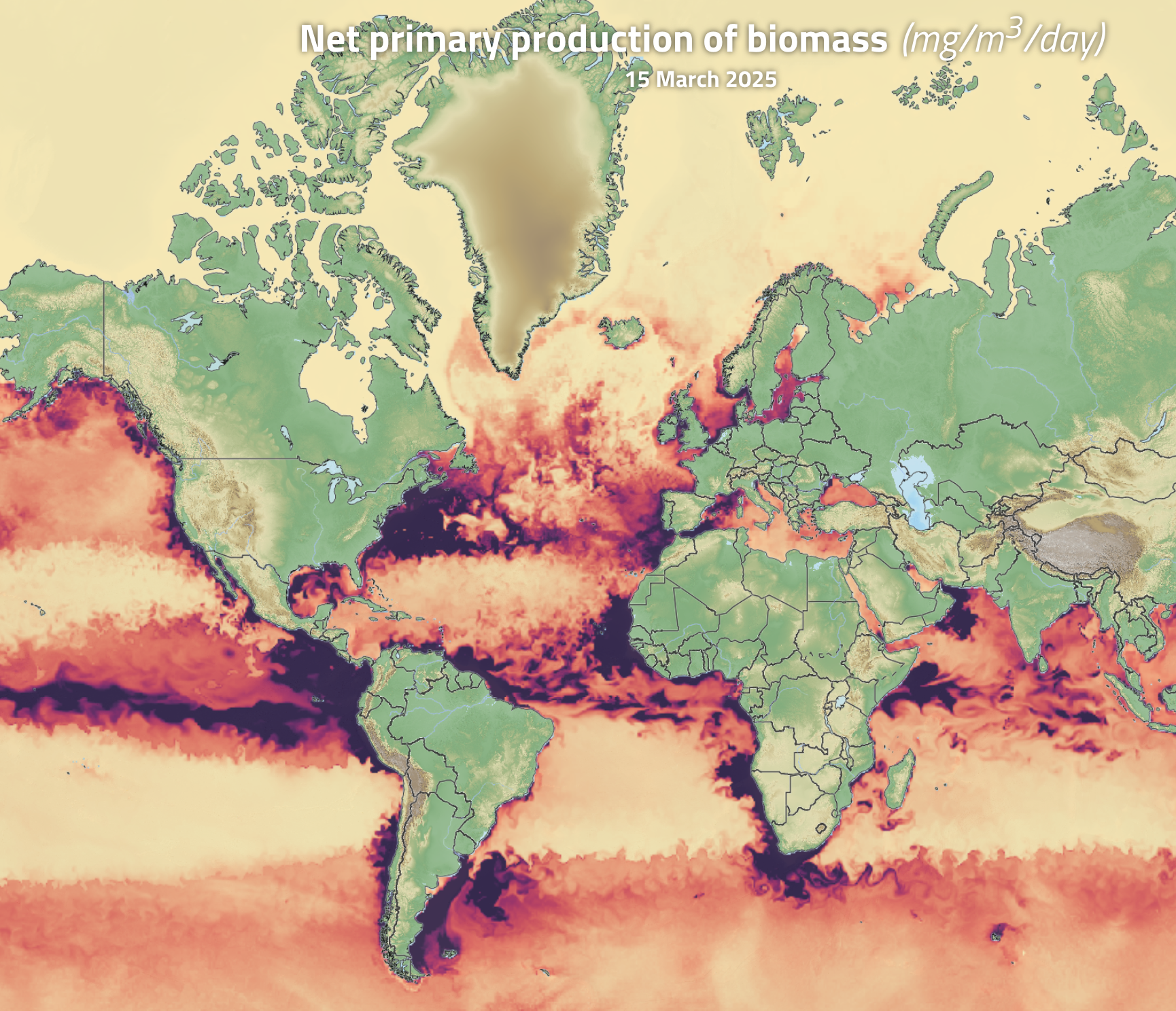] .font50[copernicus.eu] --- - Computation enables analyses that were previously impossible (permutation tests, Bayesian statistics, next-gen sequencing) .image50[] .font50[R package BNViewer] --- - Enables the creation by non-artists of **highly effective visualisations** .image70[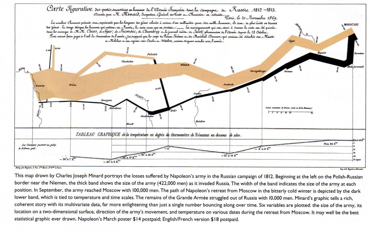] .font50[Edward R Tufte. *The Visual Display of Quantitative Information*] --- layout: true # Why/what is R? .rt30[ .rt[ [](https://cran.r-project.org) ]] --- class: .lt70 - Open-source **domain-specific** language -- - Scientific computing is built-in -- - Large number of packages specifically oriented around statistics, data science, visualisation -- - Standard language for statistics, and (to a lesser extent) bioinformatics -- - Excellent tools for scientific communication - *Rmarkdown* for websites, reports, presentations - *Shiny* for webapps --- layout: false # Course objectives - Learn fundamental concepts of R programming -- * RStudio IDE -- * Key programming concepts -- * Planning, structuring, debugging -- * Good scientific computiung practises -- - Data visualisation -- - Basic data science --- This course is for beginners! No programming experience is needed -- We will *not* cover statistical theory or advanced concepts in computer science --- # Course Format - Brief lectures to introduce general concepts (< 1 hour per session) - Structured exercises to get you coding in R -- ### Grading - Participation in class, working on exercises (40%) - Submission of a (group) report on the exercises (60%) --- # Resources & Materials - [Course web page](https://ltalluto.github.io/ue_intro_r) - Getting help: [stackoverflow.com](stackoverflow.com), R help files, **avoid chatGPT**. ### You will need - (recommended): your own laptop (you can also use university computers) - Extra time outside class to finish exercises (if needed) --- # Introduction to programming in R --- # The R environment * `R` is two things: 1. A statistical programming language 2. A software package implementing the R language (available at [https://cran.r-project.org/](https://cran.r-project.org/)) * `RStudio` is a comprehensive working environment for R ([https://rstudio.com/products/rstudio/](https://rstudio.com/products/rstudio/)) - An editor, for writing R programs - Tools to help you write and analyse code - An R console and interpreter --- layout: true # Parts of RStudio --- After launching Rstudio, create a new R **script** using the button in the upper left .image50[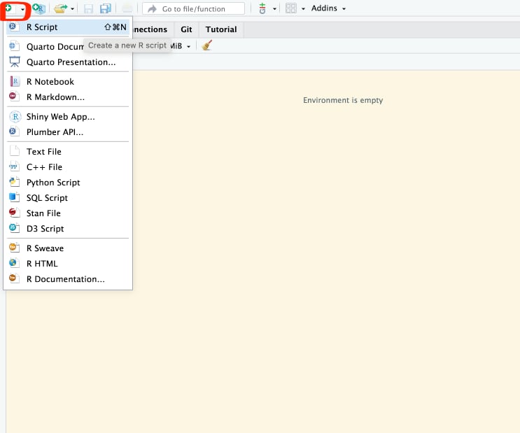] **Script**: a text file where you will write an R-program. Commands in a script will be run in order, from the top to the bottom. --- * The **editor** pane is where you will write your scripts. * Execute commands by using **run** (control-return `\(^1\)`) .image60[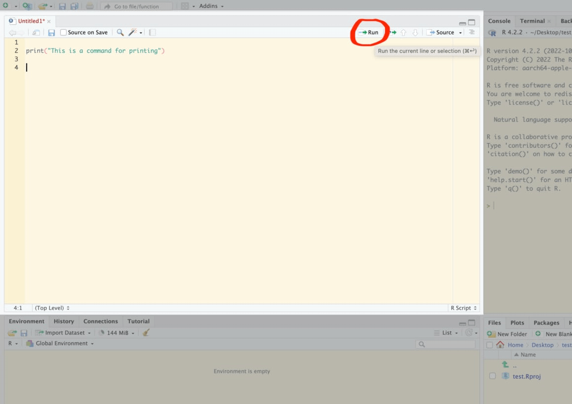] `\(^1\)`Mac users: usually you can substitute the command (&#8984;) key for control, and option for alt --- * The **console** pane is where commands are executed. .image60[  ] --- layout: false # Helpful Vocabulary * **console**: A window where you can type commands and view (text) results and output * **interpreter**: Software that translates R commands into instructions for your computer in real time * **script**: a text file containing a program, or series of commands - can be run **interactively** (sending commands one at a time to the console) - or in **batch mode** (all commands run, one after the other) * **working directory**: location on your computer where R will search for files, data, etc. --- # Organising scientific projects * Create a project in RStudio to organise your work (File => New Project) * Store all files in the project folder (your project will be **self-contained**). * Filenames: ASCII letters (No accents), numbers, underscores (_) ONLY --- # Project folder/file structure .image40[] --- # Preparing your data * Prepare data in excel * The first row is a header with column names * Column names should be **legal variable names** * In a separate file, describe the dataset, how it was collected, and the meaning of each column (including units!) * Arrange your data so that each row is a single observation, each column is a variable ("tidy" data) --- layout: true # The working directory Your **working directory** is the folder where R will look for files, folders, data. --- * It is displayed at the top of the **Console** window. * You can also type `getwd()` in the console .image80[] --- * Usually set this to the **project root directory** * It is set automatically for you if you open R by double-clicking the `project_name.Rproj` file .image80[] --- * Change it in the `Files` pane under `More` * Or use `setwd("path/to/new/folder")` in the console. .image80[] --- layout: false # Variables * A **variable** is a name that points to some data. * Variable names can contain lower- or upper-case letters, numbers, and the `_` symbol. * Names must start with letters and (when possible) should be descriptive * Variables are given values by **assignment** using either the `=` or `<-` symbol ``` r # Comments in R start with the # symbol # Legal variable names x = 1 y0 = 5 time_of_day = "20:15" dayOfWeek <- "Monday" ``` --- # Variables ### Recommendations * Use descriptive variable names instead of comments. * Avoid 1- and 2- letter names. * Separate words with underscores. * Use a consistent assignment operator (`=` or `<-`) ``` r # bad! # d is the diversity in our site, in species d = 8 # better! site_diversity = 8 ``` --- layout: true # Data types `numeric` — `integer` — `logical` — `character` — `factor` --- The **type** of a variable tells us what kind of information it contains. * **numeric**: integers and floating-point (decimal) numbers * **integer**: a special case of numeric variable * **logical**: yes/no, true/false data; in R represented by the special values `TRUE` and `FALSE` * **character**: strings, text * **factor**: special variable type for categorical (nominal & ordinal) data --- Useful functions for querying a data type are `class()` and `mode()`. ``` r x = "a string" mode(x) ## [1] "character" ``` ``` r y = 5.5 mode(y) ## [1] "numeric" ``` --- Convert between data types using `as` ``` r y = 5.5 as(y, "integer") ## [1] 5 ``` --- layout: true # Operators **Operators** perform computations on variables and constants. --- * The **assignment operators** give a value to a variable - `=`, `<-` - Both work mostly the same, use alt-dash (-) for `<-` ``` r # assignment x = 5 ``` --- * **Mathematical operators** allow us to do arithmetic - `+`, `-`, `*`, `/`, `^` ``` r # math x + 2 ## [1] 7 ``` ``` r (3 + x) * 2 ## [1] 16 ``` ``` r 3^2 ## [1] 9 ``` --- layout: true # Functions **Functions** allow for more complex operations on data --- * Functions take **arguments** inside the brackets `()` * arguments can be variables or constants ``` r x = 16 sqrt(x) ## [1] 4 ``` ``` r sqrt(25) ## [1] 5 ``` --- * Separate multiple arguments with a comma * Clarify your code by **naming** the arguments - see the help files (here: `?log`) to learn argument names! ``` r x = 100 log(x) ## [1] 4.60517 ``` -- ``` r log(x, base = 10) ## [1] 2 ``` --- layout: true # Vectors Group multiple values of the same type together in a **vector**. --- * create a vector with the concatenate function `c()`. ``` r five_numbers = c(3, 2, 8.6, 4, 9.75) print(five_numbers) ## [1] 3.00 2.00 8.60 4.00 9.75 ``` --- * Create a sequence of integers with the `:` operator ``` r one_to_ten = 1:10 print(one_to_ten) ## [1] 1 2 3 4 5 6 7 8 9 10 ``` ``` r class(one_to_ten) ## [1] "integer" ``` --- * Create arbitrary sequences using `seq()` * Repeat a value using `rep()` ``` r seq(1, 5, 0.5) ## [1] 1.0 1.5 2.0 2.5 3.0 3.5 4.0 4.5 5.0 ``` ``` r rep(0, 5) ## [1] 0 0 0 0 0 ``` --- layout: false # Vectorized operations * Many of R's basic operators and functions are **vectorized**: they apply one-at-a-time to the whole vector. ``` r five_numbers = c(3, 2, 8.6, 4, 9.75) # math on vectors is performed on each element five_numbers + 1 ## [1] 4.00 3.00 9.60 5.00 10.75 ``` ``` r five_numbers^2 ## [1] 9.0000 4.0000 73.9600 16.0000 95.0625 ``` ``` r sin(five_numbers) ## [1] 0.1411200 0.9092974 0.7343971 -0.7568025 -0.3195192 ``` --- layout: true # Indexing We can use **indexing** with the `[]` operator to get a part of a vector by its position --- ``` r five_numbers = c(3, 7, 8.6, 4, 9.75) five_numbers[3] ## [1] 8.6 ``` --- * The index itself can be a vector! ``` r five_numbers = c(3, 7, 8.6, 4, 9.75) five_numbers[2:3] ## [1] 7.0 8.6 ``` ``` r five_numbers[c(2,5)] ## [1] 7.00 9.75 ``` --- * Any legal **expression** that returns integers can be used inside `[]`! ``` r i = 1 five_numbers = c(3, 7, 8.6, 4, 9.75) five_numbers[i + 2] ## [1] 8.6 ``` --- layout: false # Reading data .lt70[ * Use `read.csv()` to read in a csv file, or `read.table()` for tab- or space-delimited files. * Here I read in the [Palmer Penguins dataset](https://github.com/allisonhorst/palmerpenguins/) ] .rt30[] .lt100[ ``` r # read.csv will also accept a url! # url = "https://raw.githubusercontent.com/allisonhorst/ # palmerpenguins/main/inst/extdata/penguins.csv" # penguins = read.csv(url) penguins = read.csv("data/penguins.csv") ``` ] --- layout: true # Data frames A **data frame** is a data structure for tabular data --- * `head()` shows the first few rows of a data frame * `View()` will open the data frame in a spreadsheet-like viewer ``` r head(penguins) ## species island bill_length_mm bill_depth_mm flipper_length_mm body_mass_g ## 1 Adelie Torgersen 39.1 18.7 181 3750 ## 2 Adelie Torgersen 39.5 17.4 186 3800 ## 3 Adelie Torgersen 40.3 18.0 195 3250 ## 4 Adelie Torgersen NA NA NA NA ## 5 Adelie Torgersen 36.7 19.3 193 3450 ## 6 Adelie Torgersen 39.3 20.6 190 3650 ## sex year ## 1 male 2007 ## 2 female 2007 ## 3 female 2007 ## 4 <NA> 2007 ## 5 female 2007 ## 6 male 2007 ``` --- * Each row in a data frame is a single **case** * Each column is a single variable, stored as a **vector** ``` r head(penguins) ## species island bill_length_mm bill_depth_mm flipper_length_mm body_mass_g ## 1 Adelie Torgersen 39.1 18.7 181 3750 ## 2 Adelie Torgersen 39.5 17.4 186 3800 ## 3 Adelie Torgersen 40.3 18.0 195 3250 ## 4 Adelie Torgersen NA NA NA NA ## 5 Adelie Torgersen 36.7 19.3 193 3450 ## 6 Adelie Torgersen 39.3 20.6 190 3650 ## sex year ## 1 male 2007 ## 2 female 2007 ## 3 female 2007 ## 4 <NA> 2007 ## 5 female 2007 ## 6 male 2007 ``` --- * `str()` gives you a summary of the **str**ucture of the data ``` r str(penguins) ## 'data.frame': 344 obs. of 8 variables: ## $ species : chr "Adelie" "Adelie" "Adelie" "Adelie" ... ## $ island : chr "Torgersen" "Torgersen" "Torgersen" "Torgersen" ... ## $ bill_length_mm : num 39.1 39.5 40.3 NA 36.7 39.3 38.9 39.2 34.1 42 ... ## $ bill_depth_mm : num 18.7 17.4 18 NA 19.3 20.6 17.8 19.6 18.1 20.2 ... ## $ flipper_length_mm: int 181 186 195 NA 193 190 181 195 193 190 ... ## $ body_mass_g : int 3750 3800 3250 NA 3450 3650 3625 4675 3475 4250 ... ## $ sex : chr "male" "female" "female" NA ... ## $ year : int 2007 2007 2007 2007 2007 2007 2007 2007 2007 2007 ... ``` --- * `nrow()`, `ncol()` and `dim()` give you data frame dimensions ``` r nrow(penguins) ## [1] 344 ``` ``` r ncol(penguins) ## [1] 8 ``` ``` r dim(penguins) ## [1] 344 8 ``` --- Data frame variables are normally **hidden** ``` r str(penguins) ## 'data.frame': 344 obs. of 8 variables: ## $ species : chr "Adelie" "Adelie" "Adelie" "Adelie" ... ## $ island : chr "Torgersen" "Torgersen" "Torgersen" "Torgersen" ... ## $ bill_length_mm : num 39.1 39.5 40.3 NA 36.7 39.3 38.9 39.2 34.1 42 ... ## $ bill_depth_mm : num 18.7 17.4 18 NA 19.3 20.6 17.8 19.6 18.1 20.2 ... ## $ flipper_length_mm: int 181 186 195 NA 193 190 181 195 193 190 ... ## $ body_mass_g : int 3750 3800 3250 NA 3450 3650 3625 4675 3475 4250 ... ## $ sex : chr "male" "female" "female" NA ... ## $ year : int 2007 2007 2007 2007 2007 2007 2007 2007 2007 2007 ... ``` ``` r print(bill_length_mm[1:5]) ## Error in eval(expr, envir, enclos): object 'bill_length_mm' not found ``` --- layout: false # Indexing with $ You can use the `$` operator to access a single variable *within* a data frame ``` r print(bill_length_mm[1:5]) ## Error in eval(expr, envir, enclos): object 'bill_length_mm' not found ``` ``` r print(penguins$bill_length_mm[1:5]) ## [1] 39.1 39.5 40.3 NA 36.7 ``` --- # The with function The `with()` function is a special function that makes data frame variables visible insde the `{}` operator ``` r with(penguins, { bill_length_mm[1:5] + bill_depth_mm[1:5] }) ## [1] 57.8 56.9 58.3 NA 56.0 ``` --- layout: true # Data frame subsets * You can use the `subset` function to extract part of a data frame that meet certain **conditions** --- * The `==` operator *tests* if two things are equal ``` r penguins_gentoo_only = subset(penguins, species == "Gentoo") head(penguins_gentoo_only) ## species island bill_length_mm bill_depth_mm flipper_length_mm body_mass_g ## 153 Gentoo Biscoe 46.1 13.2 211 4500 ## 154 Gentoo Biscoe 50.0 16.3 230 5700 ## 155 Gentoo Biscoe 48.7 14.1 210 4450 ## 156 Gentoo Biscoe 50.0 15.2 218 5700 ## 157 Gentoo Biscoe 47.6 14.5 215 5400 ## 158 Gentoo Biscoe 46.5 13.5 210 4550 ## sex year ## 153 female 2007 ## 154 male 2007 ## 155 female 2007 ## 156 male 2007 ## 157 male 2007 ## 158 female 2007 ``` --- * The `>` and `<` operators test greater-than and less-than ``` r penguins_big = subset(penguins, body_mass_g > 6000) head(penguins_big) ## species island bill_length_mm bill_depth_mm flipper_length_mm body_mass_g ## 170 Gentoo Biscoe 49.2 15.2 221 6300 ## 186 Gentoo Biscoe 59.6 17.0 230 6050 ## sex year ## 170 male 2007 ## 186 male 2007 ```