The German Tank Problem (MCMC Edition)
28.11.2023
1. Optional. Implement your own Metropolis algorithm
See the bottom of this page for some scaffolding code to get you started. Fill in the appropriate places with the code for making the algorithm work. Alternatively, there is an implementation provided on the github repository.
2. German Tank Problem
Recall the German tank problem presented in lecture. Use the following captured serial numbers:
s = c(147, 126, 183, 88, 9, 203, 16, 10, 112, 205)Your goal is to estimate a single parameter, \(N\), the highest possible serial number (indicating the number of tanks actually produced).
- What likelihood function is appropriate? Can you write this as an equation? The likelihood function should be \(pr(s|N)\).
We should use a uniform likelihood, with a minimum of 1 and \(N\) as the maximum.
\[ pr(s|N) = \frac{1}{N - 1} \quad\text{for all } 1 \le s \le N \]
- Translate this likelihood function into R code, and plot the function for varying values of \(N\).
# we do the log liklihood, better for computational reasons
#' Log liklihood function for german tank problem
#' @param N Parameter, maximum serial number possible
#' @param x Data, vector of observed serial numbers
#' @return Log liklihood of x|N
ll = function(N, x) sum(dunif(x, 1, N, log = TRUE))

# now plot it, back-transforming to see the liklihood instead of ll
N_plot = seq(1, 500, 1)
lN = exp(sapply(N_plot, ll, x = s)) # sapply because ll wants to work on ONE value of N at a time
## Warning in dunif(x, 1, N, log = TRUE): NaNs producedplot(N_plot, lN, type = 'l', bty = 'n', xlab = "N", ylab= "pr(s|N)")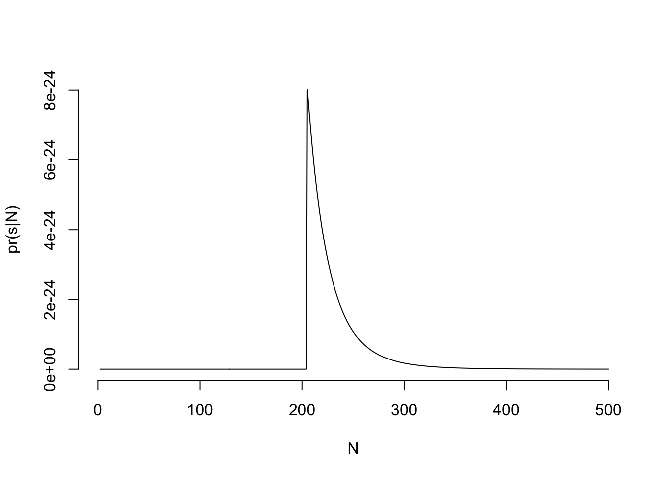
- Translate
aandbabove into a Stan statement for themodelblock. It will look something likes ~ ...
model {
    s ~ uniform(1, N);
}- Add a prior for \(N\) to your Stan
program. What prior is reasonable? Bonus: Write a prior
and posterior function in R, and plot them as in part
a.
We cannot consider \(s\) when building our prior. All that’s left is to think what is reasonable. Some knowns:
- \(N\) must be a positive number. This suggests a Gamma or Exponential prior, or a half normal. I will go with the exponential, since it is less informative than the normal and similar to the gamma, but with only one parameter instead of two for simplicity.
- In my opinion, it’s unlikely that a million tanks were produced, a billion is essentially impossible, but 10,000 is somewhat plausible.
From these two, some trial and error led me to a prior that apportions probability mass in a way that follows my beliefs.
model {
    s ~ uniform(1, N);
    N ~ exponential(0.01);
}
What does this prior tell us about different values of N?
lp = function(N, lam) dexp(N, lam, log = TRUE)

# first try prior with rate of 0.01, as in the stan code
lp(N = 100, lam = 0.01) - lp(N = 1e6, lam = 0.01)
## [1] 9999Production of 100 tanks is about 10.000 times more likely than the production of a million tanks
# Make the prior 10x less informative by adding a zero to the rate
lp(N = 100, lam = 0.001) - lp(N = 1e6, lam = 0.001)
## [1] 999.9#' Log posterior function for german tank problem
#' @param N Parameter, maximum serial number possible
#' @param x Data, vector of observed serial numbers
#' @param lam Prior rate parameter for N
#' @return Log unnormalised posterior, proportional to the probability of N|x
lpost = function(N, x, lam) ll(N, x) + lp(N, lam)
cols = scales::hue_pal()(3)
post_N = exp(sapply(N_plot, lpost, x = s, lam = 0.01))## Warning in dunif(x, 1, N, log = TRUE): NaNs producedprior_N = exp(lp(N_plot, lam = 0.01))
par(mfrow=c(2,3))
plot(N_plot, lN, type = 'l', bty = 'n', col = cols[1], xlab = "N", ylab = "pr(s|N)")
plot(N_plot, post_N, col = cols[2], lty=2, xlab = "N", type = 'l', ylab = "Unnormalised posterior")
plot(N_plot, prior_N, col = cols[3], xlab = "N", ylab = "pr(N)", type = 'l')
# The probs are not as useful sometimes as viewing them on the log scale
plot(N_plot, log(lN), type = 'l', bty = 'n', col = cols[1], xlab = "N", ylab = "pr(s|N)")
plot(N_plot, log(post_N), col = cols[2], lty=2, xlab = "N", type = 'l', ylab = "Unnormalised posterior")
plot(N_plot, log(prior_N), col = cols[3], xlab = "N", ylab = "pr(N)", type = 'l')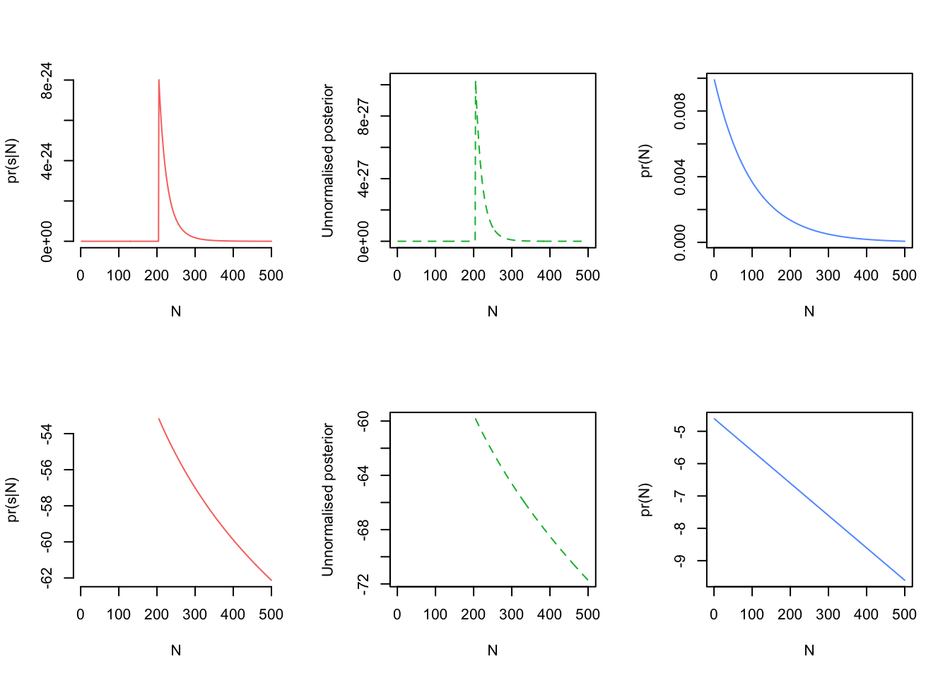
- Finish the Stan program, then use it to get the MAP estimate for N
using the
optimizingfunction. What’s the MAP estimate?- Hint: You will need to use the
vectordatatype, which we haven’t seen yet. Look it up in the Stan manual to see if you can understand how and where to use it.
- Hint: You will need to use the
data {
    int nobs; // number of observations
    vector <lower = 1> [nobs] s;
    real <lower = 0> lam; // prior hyperparameter for N
}
parameters {
    real <lower = max(s)> N; // important! N must be greater than the largest value in s
}
model {
    s ~ uniform(1, N);
    N ~ exponential(lam);
}
tank_mod = rstan::stan_model("my_stan/tank_model.stan")The above assumes you have created the stan program and saved it in a
file named "my_stan/tank_model.stan". Adjust as
appropriate.
tank_data = list(
    nobs = length(s),
    s = s,
    lam = 0.01
)
(tank_map = rstan::optimizing(tank_mod, data = tank_data)$par)
## N
## 2053. Sampling the posterior
Use sampling() to get 5000 samples from the posterior
distribution. Alternatively, if you finished part 1 above, try this with
your own sampler.
library(rstan)
tank_fit = sampling(tank_mod, data = tank_data, iter = 5000, chains = 1, refresh = 0)
tank_fit
## Inference for Stan model: anon_model.
## 1 chains, each with iter=5000; warmup=2500; thin=1;
## post-warmup draws per chain=2500, total post-warmup draws=2500.
##
## mean se_mean sd 2.5% 25% 50% 75% 97.5% n_eff Rhat
## N 223.95 0.70 20.71 205.36 210.24 217.81 230.02 278.81 886 1.00
## lp__ -53.95 0.04 0.84 -56.61 -54.11 -53.62 -53.42 -53.37 467 1.01
##
## Samples were drawn using NUTS(diag_e) at Fri Nov 29 14:10:24 2024.
## For each parameter, n_eff is a crude measure of effective sample size,
## and Rhat is the potential scale reduction factor on split chains (at
## convergence, Rhat=1).- Evaluate your samples using
mcmc_trace()andmcmc_hist()from thebayesplotpackage (or implement your own versions). You might need to useas.arrayoras.matrixto convert the samples from stan to something that bayesplot can use. Compare the histogram of samples to the posterior density plot you made in 2d.
library(bayesplot)
tank_samps = as.matrix(tank_fit)
# mcmc_combo puts multiple plots on the same figure
# What is lp__??
mcmc_combo(tank_samps, combo = c("trace", "hist"))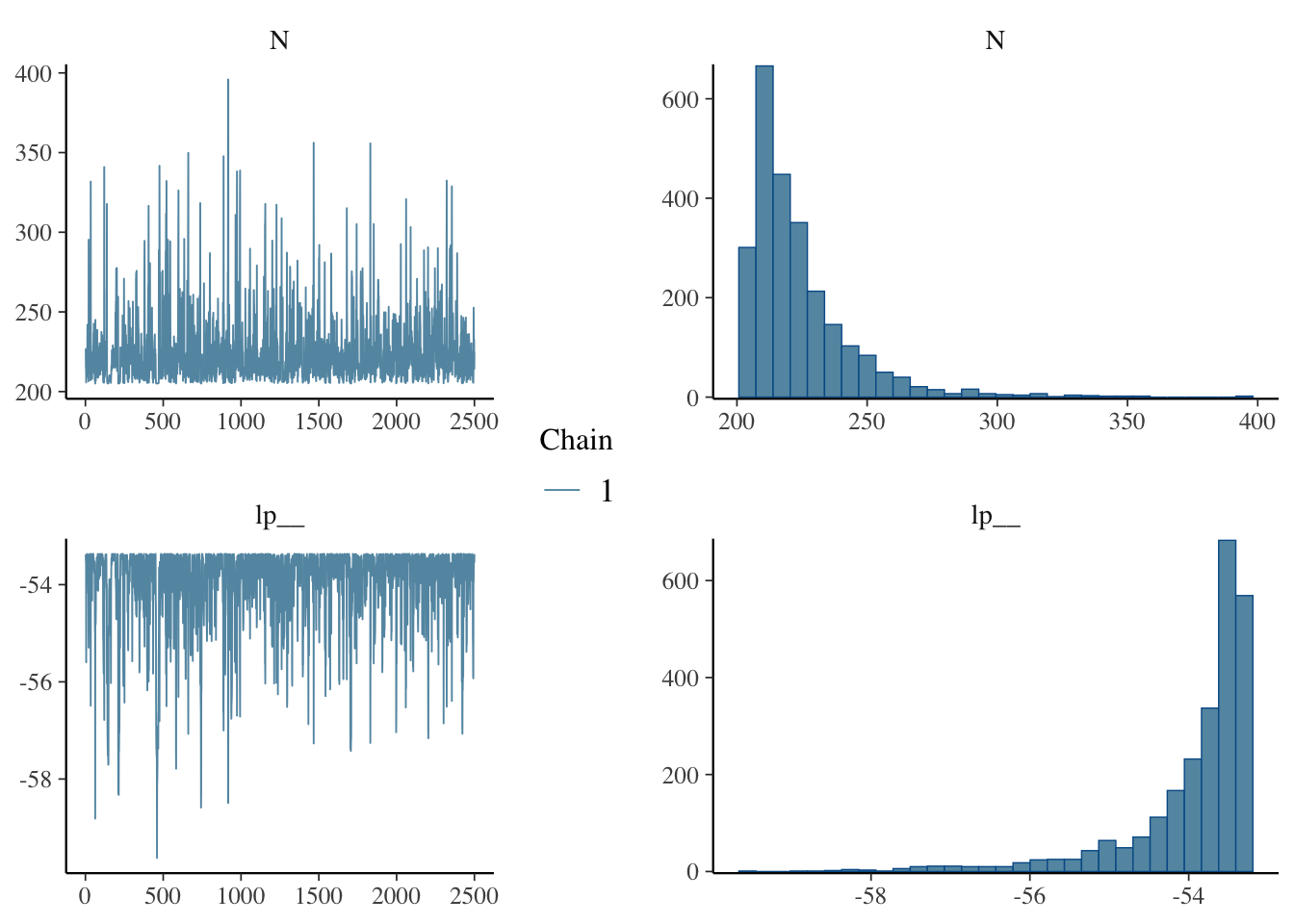
- What summary statistics can we get from the samples? How do your estimates of central tendency (mean, median, etc) compare with the MAP? What metrics of dispersion might be useful? Can you imagine how you might calculate a credible interval (== Bayesian confidence interval)?
I suggest median for this dataset, since the distribution is highly skewed.
c(mean = mean(tank_samps[,'N']), median = median(tank_samps[,'N']), mode = tank_map)## mean median mode.N
## 223.9510 217.8061 205.0000Credible intervals are tricky. We can of course construct a quantile interval:
(quant_interval = quantile(tank_samps[,'N'], c(0.05, 0.95)))## 5% 95%
## 205.8410 262.2624But this has the strange property that the mode is not included. Depending on how skewed the posterior is, it is even possible that the median is not included!
A better approach is to include the tallest 90%, which is also the narrowest interval. Such an interval is called the highest density interval (HDI). A simple approach to this is to compute many potential intervals, and choose the narrowest.
# Operate on sorted samples
# this makes it easy to take a 90% intervals from any start point: it's just the next 90% of observations
samps_sorted = sort(tank_samps[,'N'])

# how many values in a 90% interval?
int_width = ceiling(0.9 * length(samps_sorted))

# initial interval to test
interval = c(samps_sorted[1], samps_sorted[1 + int_width])

# what are the possible lower starting points for intervals
# our maximum possible start the length minus the interval width
possible_intervals = 2:(length(samps_sorted) - int_width)
for(i in possible_intervals) {
    width = interval[2] - interval[1]
    new_interval = c(samps_sorted[i], samps_sorted[i + int_width])
    new_width = new_interval[2] - new_interval[1]
    if(new_width < width)
        interval = new_interval
}

# compare with the quantile interval
intervals = rbind(quantile = quant_interval, hdi = interval)
colnames(intervals) = c("lower", "upper")
intervals
## lower upper
## quantile 205.8410 262.2624
## hdi 205.0124 248.4648The HDI is quite a bit narrower than the quantile interval.
In the git repository, there is a function that will do this for you
(including for multivariate problems):
vu_advstats_students/r/hdi.r
source("../vu_advstats_students/r/hdi.r")
hdi(tank_samps[,'N'], density = 0.9)
## lower upper
## [1,] 205.0124 248.4648Bonus: discrete uniform parameters
You probably have produced a model in 2 that treats N as a continuous varible, resulting of course in estimates that say something like “1457.3 tanks were produced.” This is of course impossible, \(N\) and \(s\) are both discrete parameters. Can you design a model that respects this constraint? How do the results differ?
Discrete parameters are tricky in Stan, and sampling in discrete space doesn’t always work. We can manage it with this relatively simple problem, in part becaues the log liklihood is quite a simple exression.
data {
    int nobs; // number of observations
    vector <lower = 1> [nobs] s;
    real <lower = 0> lam; // prior hyperparameter for N
}
parameters {
    real <lower = max(s)> N_latent;
}
model {
    s ~ uniform(1, floor(N_latent));
    N_latent ~ exponential(lam);
}
generated quantities {
    // output N, which is the "real" max serial number
    // this is the value we use to compute the likelihood, and is
    // just N_latent, rounded down
    real N = floor(N_latent);
}
tank_fit_d = sampling(tank_mod_discrete, data = tank_data, iter = 5000, chains = 1, refresh = 0, control = list(max_treedepth = 20))
tank_samps_d = as.matrix(tank_fit_d)
mcmc_combo(tank_samps_d, combo = c("trace", "hist"))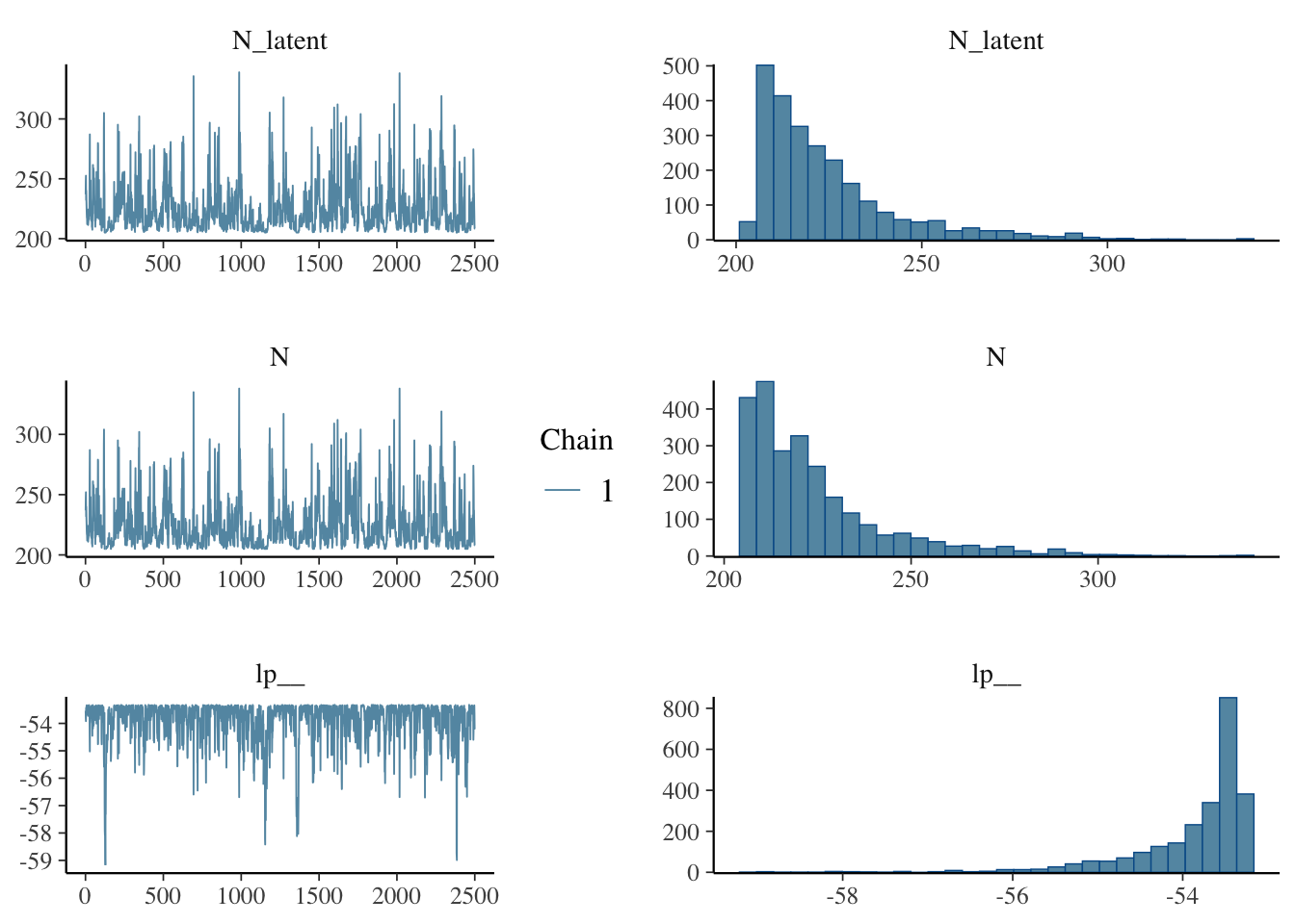
(quant_interval = quantile(tank_samps_d[,'N'], c(0.05, 0.95)))## 5% 95%
## 206 266hdi_interval = hdi(tank_samps_d[,'N'], density = 0.9)
# compare with the quantile interval
rbind(hdi = hdi_interval, quantile = quant_interval)## lower upper
## 205 250
## quantile 206 266The results are very similar, but now the mode is correctly and exactly included!