Introduction, Probability, & Distributions
Lauren Talluto
02.02.2026
Course Introduction
- Introduce ourselves - name, research area, what you want from this
course
- The course web
page has links to all code and presentations
Course Introduction
- Introduce ourselves - name, research area, what you want from this
course
- The course web
page has links to all code and presentations
- Mixture of lecture and cooperative coding
- Early in course: practise with example models
- Later in course: example models + group
projects
- Last day: status report presentations
- Important: Semi-blocked course over 3 weeks.
Significant time required outside lecture periods.
Course Introduction
This course will give you:
- A deeper understanding of how inferential statistics works
- An appreciation of the similarities between Bayesian and frequentist
methods
- The ability to think critically about model design
Course Introduction
This course will give you:
- A deeper understanding of how inferential statistics works
- An appreciation of the similarities between Bayesian and frequentist
methods
- The ability to think critically about model design
And not so much:
- A giant toolbox of ready-made models, with variations for every
potential problem
Course Introduction
Why Bayes?
Why statistics at all? What is the goal of statistical analysis?
- I want to describe some phenomenon (“model”)
- I have some general (“prior”) knowledge about the question
- I gather additional information (“data”)
Why Bayes?
Why statistics at all? What is the goal of statistical analysis?
- I want to describe some phenomenon (“model”)
- I have some general (“prior”) knowledge about the question
- I gather additional information (“data”)
What is the probability that my model is correct given
what I already know about it and what I’ve learned?
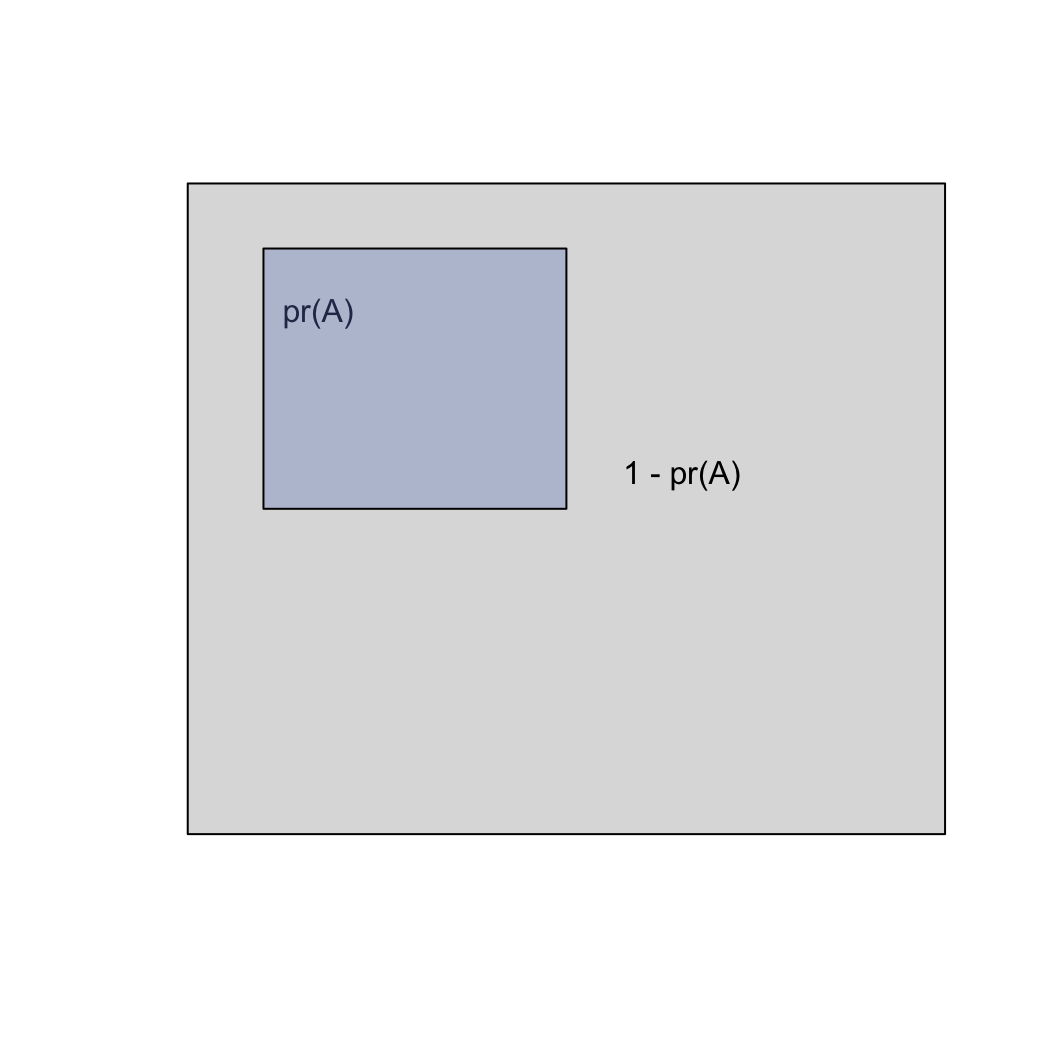
Probabilistic partitions
Imagine a box with a total area of 1, representing all possible
events
Probabilistic partitions
- An event A has some probability of occurring: pr(A)
(marginal probability)
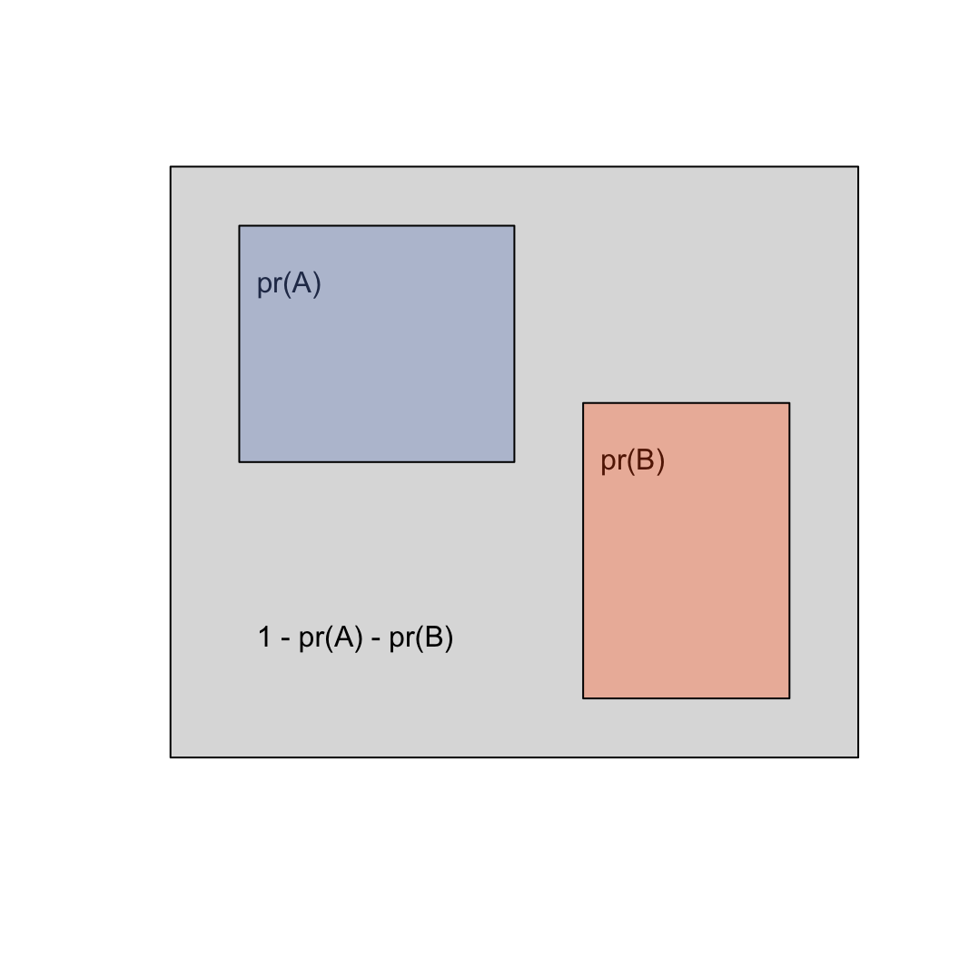
Probabilistic partitions
- An event A has some probability of occurring: pr(A)
(marginal probability)
- A second event, B, has multiple possible relationships to A.
- If A and B never occur together, the events are
disjoint
|
|
!B
|
B
|
|
!A
|
1 - pr(A) - pr(B)
|
pr(B)
|
|
A
|
pr(A)
|
0
|
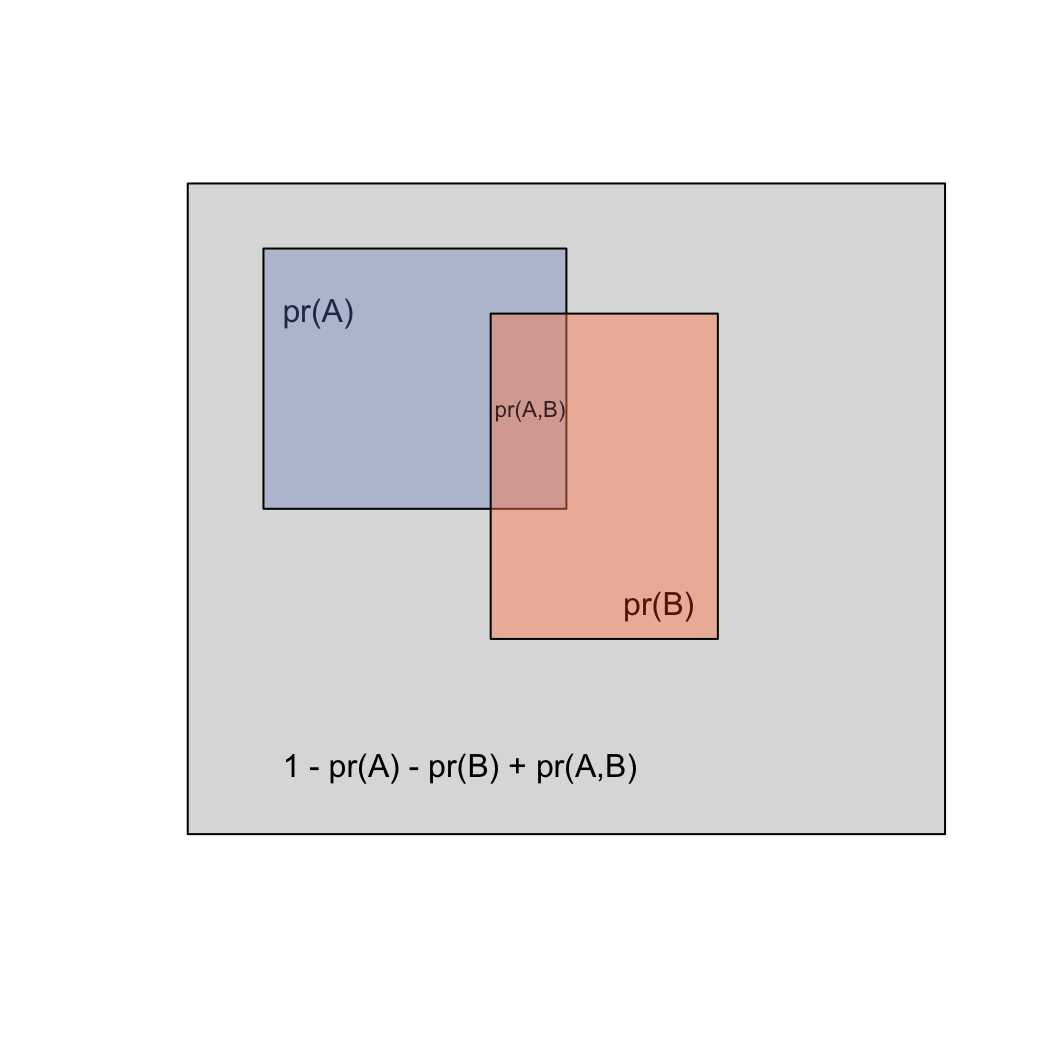
Probabilistic partitions
- An event A has some probability of occurring: pr(A)
- A second event, B, has multiple possible relationships to A:
- If A and B never occur together, the events are
disjoint
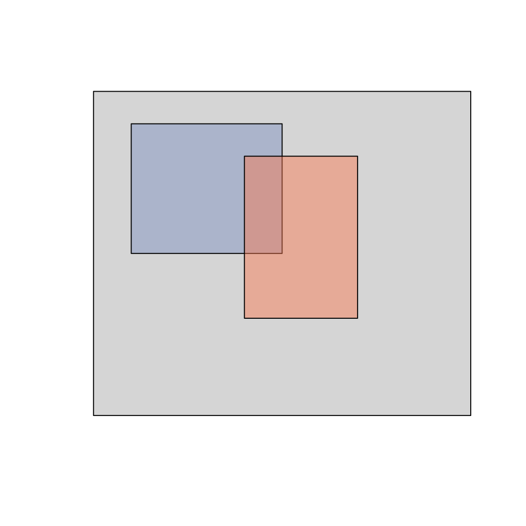
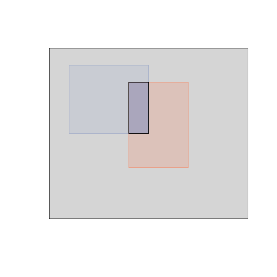
- If the two overlap, we can say that they
intersect
|
|
!B
|
B
|
|
!A
|
1 - pr(A) - pr(B) + pr(A,B)
|
pr(B) - pr(A,B)
|
|
A
|
pr(A) - pr(A,B)
|
pr(A,B)
|
Probabilistic partitions
- An event A has some probability of occurring: pr(A)
- A second event, B, has multiple possible relationships to A:
- If A and B never occur together, the events are
disjoint
- If the two overlap, we can say that they
intersect
- pr(A,B) = the probability of both (joint
probability)
- Also written \(A \cap B\) (the
intersection of A and B)
- pr(A) + pr(B) - pr(A,B) is the union (\(A \cup B\))
- the chance of at least one event
- for disjoint events, pr(A,B) = 0, so \(A \cup B = pr(A) + pr(B)\)
Independence
- A and B are independent if pr(A) is not influenced by whether B has
occurred, and vice-versa
- \(pr(A,B) = pr(A)pr(B)\)
(joint probability)
- \(pr(A|B) = pr(A)\)
- \(pr(B|A) = pr(B)\)
Conditional probability
- \(pr(A|B)\) is the probability that
\(A\) occurs, given that we already
know \(B\) has occurred
- We notate the opposite (pr that \(A\) occurs given that \(B\) has not): \(pr(A|'B)\)
- We can define conditional probabilities in terms of
joint and marginal probabilities
\[pr(A,B) = pr(A|B)pr(B)\]
So now that we have learned how to manupulate probabilities….
Can anyone define probability?
Manipulating conditional probabilities
Are you a (latent) zombie?
The problem:
People are turning into zombies! We have a test, but it is imperfect,
with a false positive rate = 1% and a false negative
rate = 0.5%.
You take the test, and the result is positive. What is the
probability that you are actually going to become a zombie?
Is probability the same as frequency?
- You took the zombie test, the result is positive (\(T\)). we want to know \(pr(Z|T)\)
- We already know \(pr(T|Z) = 0.99\):
this is the true positive rate
- We could use this along with statistical decision
theory to make a decision about our status
- So what’s our null hypothesis?
- \(H_0\): I am not a zombie! (\(Z'\))
- \(H_A\): I am a zombie! (\(Z\))
- According to the false positive rate
- \(pr(T|Z') = 1 - pr(T|Z) =
0.01\)
- \(p < 0.05\)
- Conclusion: Reject \(H_0\), I must
be a zombie
The doctor makes a decision:
She grabs a shotgun…
Hopefully (for the sake of your health), this is unsatisfying… but
why?
Another try: manipulating conditional probabilities
Are you a (latent) zombie?
The problem:
People are turning into zombies! We have a test, but it is imperfect,
with a false positive rate = 1% and a false negative
rate = 0.5%.
You take the test, and the result is positive. What is the
probability that you are actually going to become a zombie?
Let’s add some information: We also learn that 0.1% of the population
is infected.
- False positive rate = \(pr(T|Z') =
0.01\)
- False negative rate = \(pr(T'|Z) =
0.005\)
- Prevalence = \(pr(Z) = 0.001\)
Exercise: Use the probability laws we know to
compute the probability that you are a zombie.
Hints
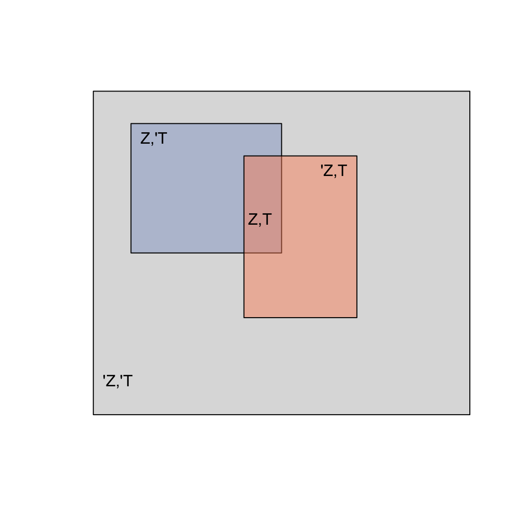
- Define the partitions:
- Zombie (\(Z\)) or not a zombie
(\('Z = 1 - Z\))
- Positive test (\(T\)) or negative
test (\('T = 1 - T\))
- Assign known numbers to statements of joint,
marginal, or conditional
probabilities
- Compute unknowns using the conditional probability rule: \(pr(A,B) = pr(A|B)pr(B)\)
- Assign concrete numbers: imagine testing 1,000,000 people. How many
are zombies? How many test positive? How many test positive and are
zombies?
Detecting Zombies
Intuitively: the test is good, so the probability that a
positive testing individual is a zombie should be high
(many
people answer 99%, given the false positive rate of 1%).
Unintuitively: zombies are very rare, so when testing many
people randomly, many tests will be false positives.
Desired outcome: \(pr(Z |
T)\)
(if I test positive, what is the probability I am a
zombie?)

Detecting Zombies — Contingency Table
- Consider a population of a million people, in a contingency
table.
Desired outcome: \(pr(Z |
T)\)
(if I test positive, what is the probability I am a
zombie?)
|
|
Test+
|
Test-
|
Sum
|
|
Zombie
|
–
|
–
|
–
|
|
Not Zombie
|
–
|
–
|
–
|
|
Sum
|
–
|
–
|
1,000,000
|
Detecting Zombies — Contingency Table
- Consider a population of a million people, in a contingency
table.
- 0.1% of the population is infected with a parasite that will
turn them into zombies (1000 zombies)
Desired outcome: \(pr(Z |
T)\)
(if I test positive, what is the probability I am a
zombie?)
|
|
Test+
|
Test-
|
Sum
|
|
Zombie
|
–
|
–
|
1,000
|
|
Not Zombie
|
–
|
–
|
999,000
|
|
Sum
|
–
|
–
|
1,000,000
|
Detecting Zombies — Contingency Table
- Consider a population of a million people, in a contingency
table.
- 0.1% of the population is infected with a parasite that will
turn them into zombies (1000 zombies)
- false negative rate = 0.5%
- 0.5% of zombies will falsely test negative: 5 negative zombies, 995
positive ones
Desired outcome: \(pr(Z |
T)\)
(if I test positive, what is the probability I am a
zombie?)
|
|
Test+
|
Test-
|
Sum
|
|
Zombie
|
995
|
5
|
1,000
|
|
Not Zombie
|
–
|
–
|
999,000
|
|
Sum
|
–
|
–
|
1,000,000
|
Detecting Zombies — Contingency Table
- Consider a population of a million people, in a contingency
table.
- 0.1% of the population is infected with a parasite that will
turn them into zombies (1000 zombies)
- false negative rate = 0.5%
- 0.5% of zombies will falsely test negative: 5 negative zombies, 995
positive ones
- false positive rate = 1%
- 1% of non-zombies will falsely test positive: 9990 positive normals,
989010 negative normals
Desired outcome: \(pr(Z |
T)\)
(if I test positive, what is the probability I am a
zombie?)
|
|
Test+
|
Test-
|
Sum
|
|
Zombie
|
995
|
5
|
1,000
|
|
Not Zombie
|
9,990
|
989,010
|
999,000
|
|
Sum
|
10,985
|
989,015
|
1,000,000
|
Detecting Zombies — Contingency Table
- Consider a population of a million people, in a contingency
table.
- 0.1% of the population is infected with a parasite that will
turn them into zombies (1000 zombies)
- false negative rate = 0.5%
- 0.5% of zombies will falsely test negative: 5 negative zombies, 995
positive ones
- false positive rate = 1%
- 1% of non-zombies will falsely test positive: 9990 positive normals,
989010 negative normals
The positive test is a given. This shrinks our world of
possibilities
- \(\frac{995}{10985}\) are zombies,
or 9.06%
Desired outcome: \(pr(Z |
T)\)
(if I test positive, what is the probability I am a
zombie?)
|
|
Test+
|
Test-
|
Sum
|
|
Zombie
|
995
|
|
|
|
Not Zombie
|
9,990
|
|
|
|
Sum
|
10,985
|
|
|
Detecting Zombies — Conditional Probabilities
- First translate numbers to probabilities
0.1% of the population is infected with a parasite that will turn
them into zombies.
- \(pr(Z) = 0.001\)
- This is the prevalence of zombies or the
prior probability that a randomly selected person is a
zombie
Desired outcome: \(pr(Z |
T)\)
(if I test positive, what is the probability I am a
zombie?)
Detecting Zombies — Conditional Probabilities
- First translate numbers to probabilities
false negative rate = 0.5%
false positive
rate = 1%
- \(pr(T' | Z) = 0.005\)
- \(pr(T | Z') = 0.01\)
Desired outcome: \(pr(Z |
T)\)
(if I test positive, what is the probability I am a
zombie?)
Given
Detecting Zombies — Conditional Probabilities
- Use probability rules to find other easy unknowns
- True positive rate:
\(pr(T | Z) = 1 - pr(T' | Z) = 1 -
0.005 = 0.995\)
\(pr(T' | Z') = 1 - pr(T | Z')
= 1 - 0.01 = 0.99\)
Desired outcome: \(pr(Z |
T)\)
(if I test positive, what is the probability I am a
zombie?)
Given
- \(pr(Z) = 0.001\)
- \(pr(T' | Z) = 0.005\)
- \(pr(T | Z') = 0.01\)
Detecting Zombies — Conditional Probabilities
- Use the product rule to compute the joint
probability
\(pr(Z,T) = pr(T|Z)pr(Z) = 0.995 \times
0.001 = 0.000995\)
- The product rule is reversible:
- \(pr(Z,T) = pr(T|Z)pr(Z) =
pr(Z|T)pr(T)\)
- Simple algebra can solve for the quantity we desire
Bayes’ Theorem
\(pr(Z|T) =
\frac{pr(T|Z)pr(Z)}{pr(T)}\)
Desired outcome: \(pr(Z |
T)\)
(if I test positive, what is the probability I am a
zombie?)
Given
- \(pr(Z) = 0.001\)
- \(pr(T' | Z) = 0.005\)
- \(pr(T | Z') = 0.01\)
Known
- \(pr(T | Z) = 0.995\)
- \(pr(T' | Z') = 0.99\)
Detecting Zombies — Bayes’ Theorem
\[pr(Z|T) =
\frac{pr(T|Z)pr(Z)}{pr(T)}\]
- We are missing a single value: \(pr(T)\)
- There are two ways to get a positive test:
- positive, and a zombie: \(pr(Z,T)\)
- positive, and not a zombie: \(pr(Z',T)\)
\[
\begin{aligned}
pr(T) & = pr(T,Z) + pr(T,Z') \\
& = pr(T|Z)pr(Z) + pr(T|Z')pr(Z') \\
& = 0.995 \times 0.001 + 0.01 \times 0.999 \\
& = 0.000995 + 0.000999 \\
& = 0.010985
\end{aligned}
\]
Desired outcome: \(pr(Z |
T)\)
(if I test positive, what is the probability I am a
zombie?)
Given
- \(pr(Z) = 0.001\)
- \(pr(T' | Z) = 0.005\)
- \(pr(T | Z') = 0.01\)
Known
- \(pr(T | Z) = 0.995\)
- \(pr(T' | Z') = 0.99\)
- \(pr(Z,T) = 0.000995\)
Detecting Zombies — Bayes’ Theorem
\[
\begin{aligned}
pr(Z|T) & = \frac{pr(T|Z)pr(Z)}{pr(T)} \\
& = \frac{0.995 \times 0.001}{0.010985} \\
& = 0.0906
\end{aligned}
\]
- Our decision theory before led us astray. Here (using decision
theory) we must reject the hypothesis that I am a
zombie (p > 0.05)!
- How could this happen?!
Desired outcome: \(pr(Z |
T)\)
(if I test positive, what is the probability I am a
zombie?)
Given
- \(pr(Z) = 0.001\)
- \(pr(T' | Z) = 0.005\)
- \(pr(T | Z') = 0.01\)
Known
- \(pr(T | Z) = 0.995\)
- \(pr(T' | Z') = 0.99\)
- \(pr(Z,T) = 0.000995\)
- \(pr(T) = 0.010985\)
Is probability the same as frequency?
- You took the zombie test, the result is positive (\(T\)). we want to know \(pr(Z|T)\)
- We already know \(pr(T|Z) = 0.99\):
this is the true positive rate
- We could use this along with statistical decision
theory to make a decision about our status
- So what’s our null hypothesis?
- \(H_0\): I am not a zombie! (\(Z'\))
- \(H_A\): I am a zombie! (\(Z\))
- According to the false positive rate
- \(pr(T|Z') = 1 - pr(T|Z) =
0.01\)
- \(p < 0.05\)
- Conclusion: Reject \(H_0\), I must
be a zombie
The doctor makes a decision:
She grabs a shotgun…
Hopefully (for the sake of your health), this is unsatisfying… but
why?
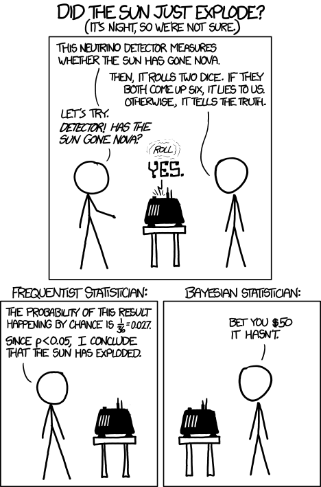
- This approach relies on the interpretation of probailities as
frequencies.
- Repeating the test across many copies of me, we would make the right
decision 95% of the time
- But I am unique! It doesn’t make sense to talk about the
frequency of zombisim in me. I either am or am not a
zombie!
- Mathematically, we want to know \(pr(Z|T)\) but we test a hypothesis about
\(pr(T|Z)\). These are not equal!
- In logic, this is known as the base rate fallacy:
we forgot about \(pr(Z)\)
- In science, this is known as the replication
crisis
So now that we have learned how to manupulate probabilities….
Can anyone define probability?
- Our degree of belief integrating all of our
knowledge
- Our problem: We only evaluate the data given a
hypothesis. We rarely ask if the hypothesis is 🐂💩
Signal detection problems
The zombie example is cute, but it is a real biological problem.
“True” state is often hidden, we have an imperfect signal.
Signal detection problems
- Desired outcome: presence/absence of endangered species
- Imperfect indicator (expert observation)
- Desire to know \(pr(present |
observed)\)
|
|
Observed
|
Not Observed
|
|
Present
|
—
|
—
|
|
Absent
|
—
|
—
|
Signal detection problems
Desired outcome: presence/absence of endangered species
Imperfect indicator (expert observation)
Desire to know \(pr(present |
observed)\)
True positive: \(pr(P|O)\):
|
|
Observed
|
Not Observed
|
|
Present
|
True positive
|
—
|
|
Absent
|
—
|
—
|
Signal detection problems
Desired outcome: presence/absence of endangered species
Imperfect indicator (expert observation)
Desire to know \(pr(present |
observed)\)
True positive: \(pr(P|O)\):
False positive: \(pr(P'|O)\):
- We misidentified a non-target species, the target species is not
present
- Many studies assume \(pr(P'|O) =
0\)
|
|
Observed
|
Not Observed
|
|
Present
|
True positive
|
—
|
|
Absent
|
False positive
|
—
|
Signal detection problems
Desired outcome: presence/absence of endangered species
Imperfect indicator (expert observation)
Desire to know \(pr(present |
observed)\)
True positive: \(pr(P|O)\):
False positive: \(pr(P'|O)\):
- We misidentified a non-target species, the target species is not
present
- Many studies assume \(pr(P'|O) =
0\)
False negative: \(pr(P|O')\):
- It’s there, but we failed to detect it
- Often referred to as the detection probability
|
|
Observed
|
Not Observed
|
|
Present
|
True positive
|
False negative
|
|
Absent
|
False positive
|
—
|
Signal detection problems
Desired outcome: presence/absence of endangered species
Imperfect indicator (expert observation)
Desire to know \(pr(present |
observed)\)
True positive: \(pr(P|O)\):
False positive: \(pr(P'|O)\):
- We misidentified a non-target species, the target species is not
present
- Many studies assume \(pr(P'|O) =
0\)
False negative: \(pr(P|O')\):
- It’s there, but we failed to detect it
- Often referred to as the detection probability
True negative: \(pr(P'|O')\):
- It’s not there, and we did not record it there
|
|
Observed
|
Not Observed
|
|
Present
|
True positive
|
False negative
|
|
Absent
|
False positive
|
True negative
|
Probability Concepts/Rules
Probability Concepts/Rules
Product rule => Chain rule
\[
\begin{aligned}
pr(A,B) & = pr(A|B)pr(B) \\
\end{aligned}
\]
Probability Concepts/Rules
Product rule => Chain rule
\[
\begin{aligned}
pr(A,B) & = pr(A|B)pr(B) \\
\end{aligned}
\]
\[
\begin{aligned}
pr(A,B,C) & = pr(A|B,C)pr(B,C) \\
& = pr(A|B,C)pr(B|C)pr(C)
\end{aligned}
\]
Probability Concepts/Rules
Product rule => Chain rule
\[
\begin{aligned}
pr(A,B) & = pr(A|B)pr(B) \\
\end{aligned}
\]
\[
\begin{aligned}
pr(A,B,C) & = pr(A|B,C)pr(B,C) \\
& = pr(A|B,C)pr(B|C)pr(C)
\end{aligned}
\]
\[
\begin{aligned}
pr(\bigcap_{k=1}^{n} A_k) & = pr(A_n | \bigcap_{k=1}^{n-1} A_k
)pr(\bigcap_{k=1}^{n-1} A_k) \\
& =\prod_{k=1}^{n}pr(A_k | \bigcap_{j=1}^{k-1}A_j)
\end{aligned}
\]
Probability Concepts/Rules
- Marginal probability: \(pr(A)\)
- Conditional probability: \(pr(A|B)\)
- Joint probability: \(pr(A,B) = pr(A \cap B)\)
Probability Concepts/Rules
- Marginal probability: \(pr(A)\)
- Conditional probability: \(pr(A|B)\)
- Joint probability: \(pr(A,B) = pr(A \cap B)\)
- Complementary rule: \(pr(A') = 1 - pr(A)\)
- Addition rule: \(pr(A
\cup B) = pr(A) + pr(B) - pr(A \cap B)\)
- For disjoint events: \(pr(A \cap
B) = 0\)
- Product rule: \(pr(A,B) =
pr(A|B)pr(B)\)
- For independent events: \(pr(A|B)
= pr(A)\)
- Chain rule: \(pr(\bigcap_{k=1}^{n} A_k) =\prod_{k=1}^{n}pr(A_k |
\bigcap_{j=1}^{k-1}A_j)\)
- Bayes’ theorem: \(pr(B|A)
= \frac{pr(A|B)pr(B)}{pr(A)}\)
What if zombies are common?
- Our test gets more useful if \(pr(Z) =
0.3\)
- Testing one person randomly taken from a (effectively) infinite
population, 30% of the time the person is a zombie
- Trivially, doing this 10 times would result in 3 zombies, 7
normals.
- But the sampling is random! Sometimes we will see 4 zombies,
sometimes 2, etc. How often?
The zombie distribution
- Generally, what is the probability of \(k\) zombies when we sample \(n\) people?
The zombie distribution
- Generally, what is the probability of \(k\) zombies when we sample \(n\) people?
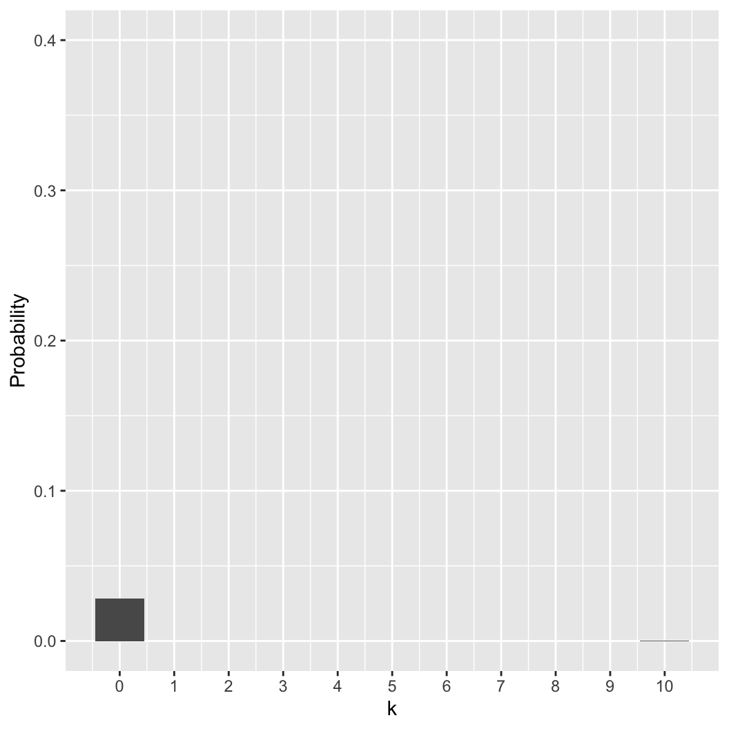
- There is only one possible way to have 10 normal people:
\[\begin{align}
pr(k = 0 | n = 10, p = 0.3) & = (0.7 \times \ldots 0.7) \\
& = 0.7^{10} \\
& \approx 0.028 \\
\end{align}\]
- The same logic applies for 10 zombies:
\[pr(k = 10 | n = 10, p = 0.3) = 0.3^{10}
\approx 0.000 \]
The zombie distribution
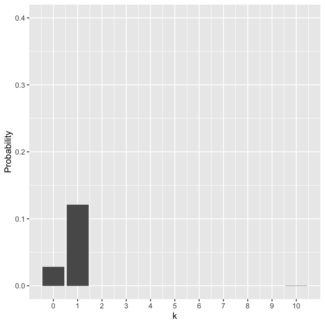
- Generally, what is the probability of \(k\) zombies when we sample \(n\) people?
- There are 10 ways to have exactly one zombie (why?).
- The probability of one of those ways:
\[pr(Z_1,Z'_{2..10}) = 0.3 \times0.7^9
\approx 0.012 \]
\[pr(k=1|n=10,p=0.3) = 10 \times 0.3
\times0.7^9 \approx 0.121\]
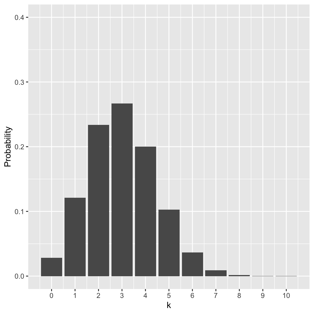
The zombie binomial distribution
- Generally, what is the probability of \(k\) zombies when we sample \(n\) people?
- The probability that we will get any one result (i.e., order
matters):
\[pr(Z_{a}, Z'_{a'}) = p^k(1 -
p)^{(n - k)}\]
- The number of different ways to achieve a given result is the
binomial function (“n choose k”)
- It follows:
\[pr(k|n,p) = {n \choose k}
p^k(1-p)^{(n-k)}\]
choose(n = 10, k = 0:10)
##  [1]   1  10  45 120 210 252 210 120  45  10   1
round(dbinom(0:10, 10, 0.3), 3)
##  [1] 0.028 0.121 0.233 0.267 0.200 0.103 0.037 0.009 0.001 0.000 0.000
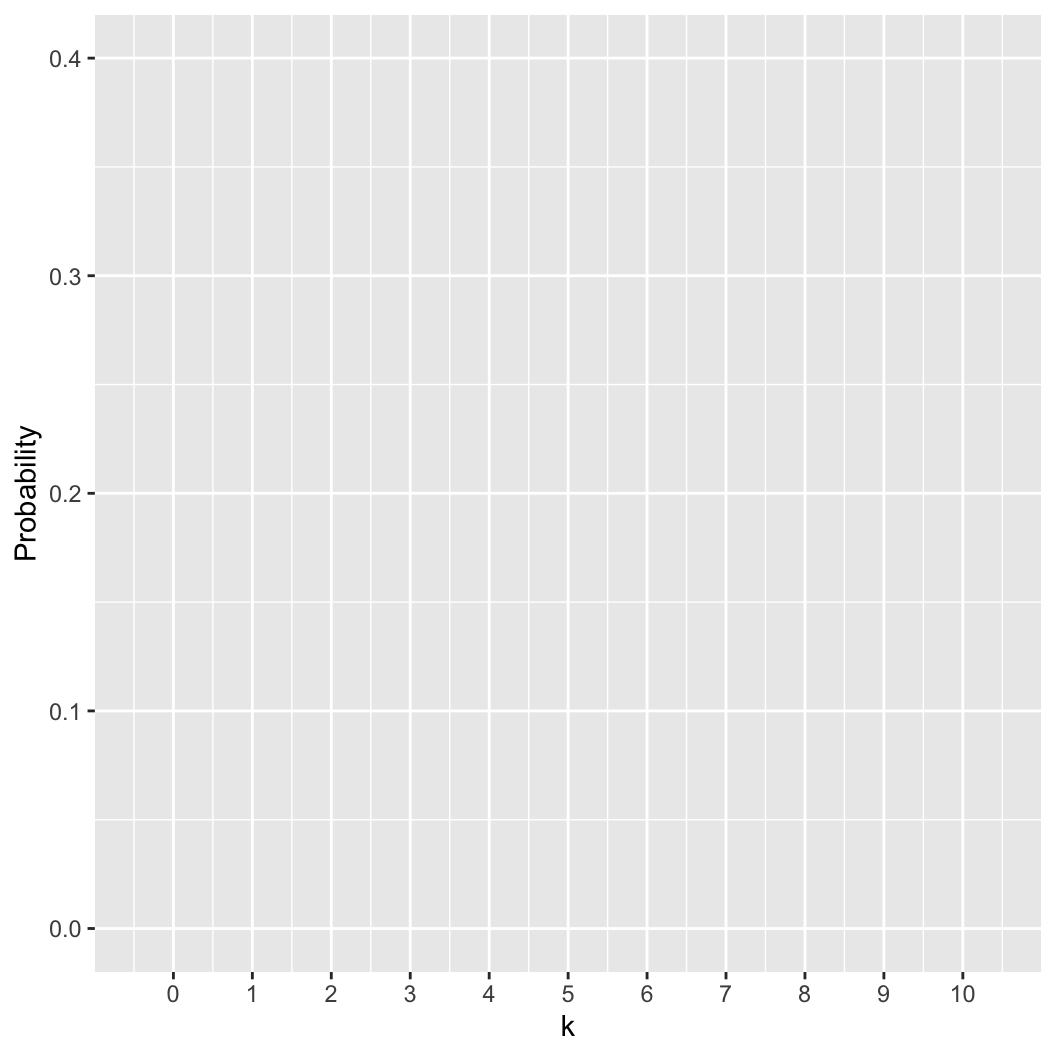
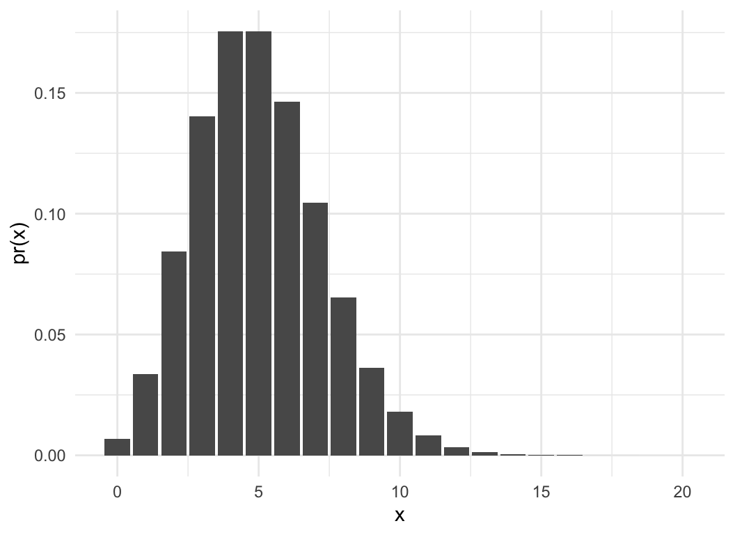
Binomial distribution
This is the probability mass function (PMF) of
the binomial distribution (dbinom in R)
\[pr(k|n,p) = {n \choose k}
p^k(1-p)^{(n-k)}\]
What is the probability of observing \(k\) events out of \(n\) independent trials, when \(pr(k) = p\)?
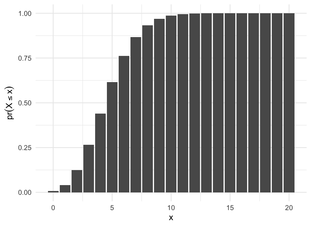
Binomial distribution
This is the probability mass function (PMF) of
the binomial distribution (dbinom in R)
\[pr(k|n,p) = {n \choose k}
p^k(1-p)^{(n-k)}\]
What is the probability of observing \(k\) events out of \(n\) independent trials, when \(pr(k) = p\)?
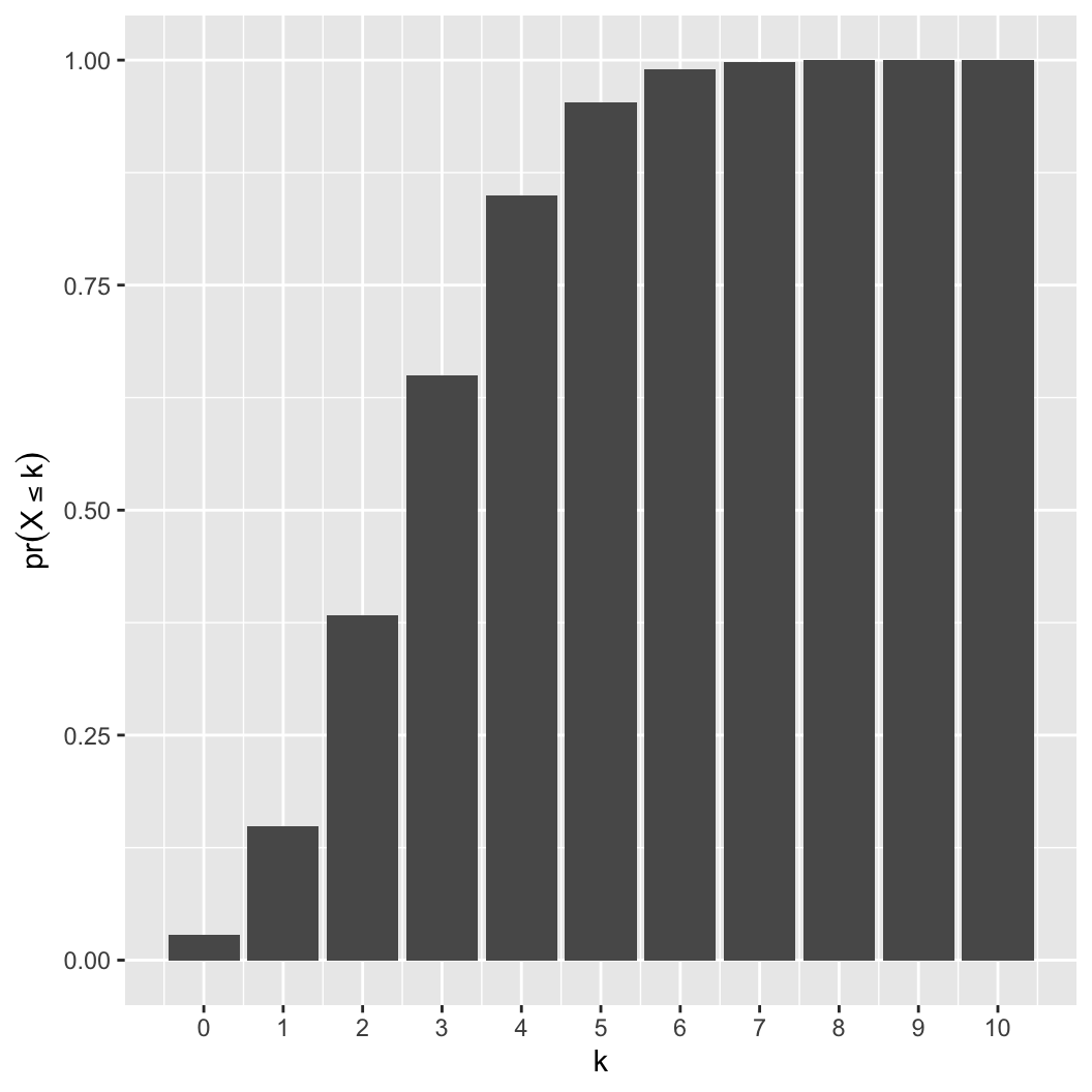
What is the probability of observing \(\le k\) events? Cumulative
distribution function (CDF)
\[
pr(X \le k|n,p) = \sum_{i=0}^{k} {n \choose i}p^i(1-p)^{(n-i)}
\]
k = 0:10
y = pbinom(k, 10, 0.3)
round(y, 3)
##  [1] 0.028 0.149 0.383 0.650 0.850 0.953 0.989 0.998 1.000 1.000 1.000
round(sum(dbinom(0:2,10,0.3)), 3)
## [1] 0.383
Poisson distribution
- Probability of observing \(x\)
events in a fixed time/space given a rate of \(\lambda\)
- Limit of binomial as \(n \rightarrow
\infty\) and \(p \rightarrow
0\)
- mean = variance = \(\lambda\)
- Commonly used for “simple” counts where \(n\) is unknown
I invent a zombie detector, it counts up every time a zombie
walks past. I put them out in busy parks. How many zombies do I
get?
lam = 5
pois_dat = data.frame(x = 0:20)
pois_dat$pmf = dpois(pois_dat$x, lam)
pois_dat$cdf = ppois(pois_dat$x, lam)
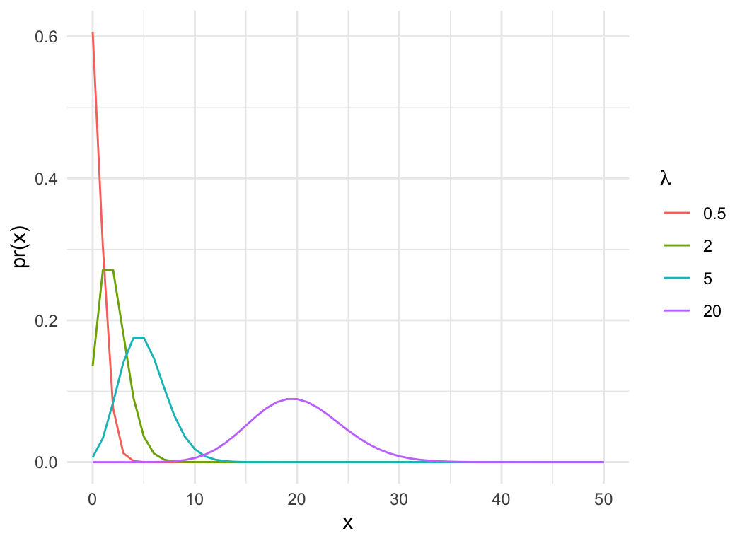
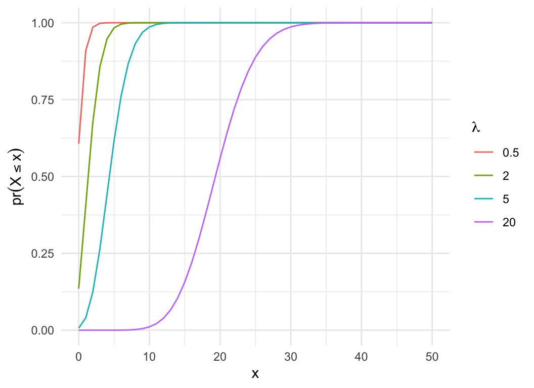
Poisson distribution
- Probability of observing \(x\)
events in a fixed time/space given a rate of \(\lambda\)
- Limit of binomial as \(n \rightarrow
\infty\) and \(p \rightarrow
0\)
- mean = variance = \(\lambda\)
- Commonly used for “simple” counts where \(n\) is unknown
I invent a zombie detector, it counts up every time a zombie
walks past. I put them out in busy parks. How many zombies do I
get?
lam = c(0.5, 2, 5, 20)
pois_dat = expand.grid(x=0:50, lam=lam)
pois_dat$pmf = dpois(pois_dat$x, pois_dat$lam)
pois_dat$cdf = ppois(pois_dat$x, pois_dat$lam)
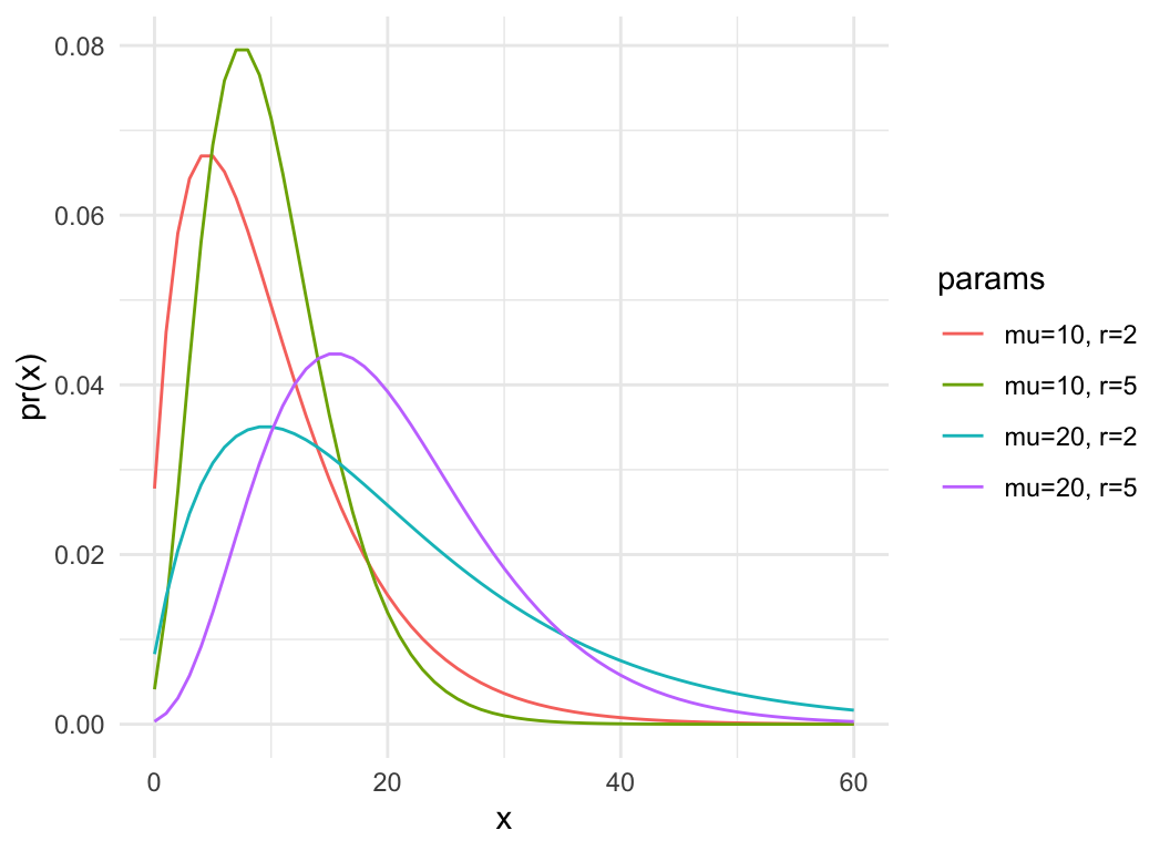
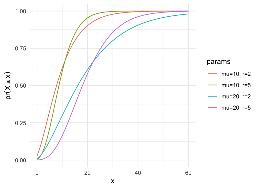
Negative binomial distribution
- Choose one person from the population where \(p = pr(Z) = 0.3\). Is she/he a zombie?
Repeat…
- How many non-zombies will I observe before I find \(r\) zombies?
- In biology, often parameterized by mean (\(\mu\)) and dispersion (\(r\)) instead of size (\(r\)) and probability (\(p\)), used for “overdispersed” counts
\[\mu = \frac{pr}{1-p}\] \[
s^2 = \mu + \frac{\mu^2}{r}
\]
dat = expand.grid(x = 0:60, mu = c(10,20), size = c(5, 2))
dat$pmf = with(dat, dnbinom(x, mu=mu, size=size))
dat$cdf = with(dat, pnbinom(x, mu=mu, size=size))
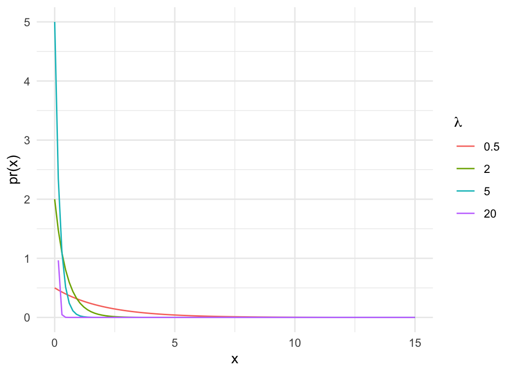
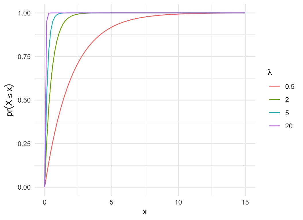
Exponential distribution
- Complement to Poisson, models the time between events of a Poisson
process with rate \(\lambda\)
- \(\mu = \frac{1}{\lambda}\)
- Continuous, defined on \((0,
\infty)\)
For a zombie detector in a park, how much time will pass between
each zombie passing by the detector?
lam = c(0.5, 2, 5, 20)
dat = expand.grid(x=seq(0,15, length.out=100), lam=lam)
dat$pdf = dexp(dat$x, dat$lam)
dat$cdf = pexp(dat$x, dat$lam)
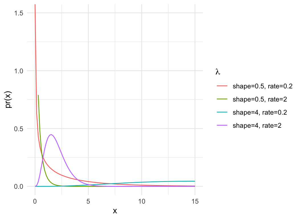
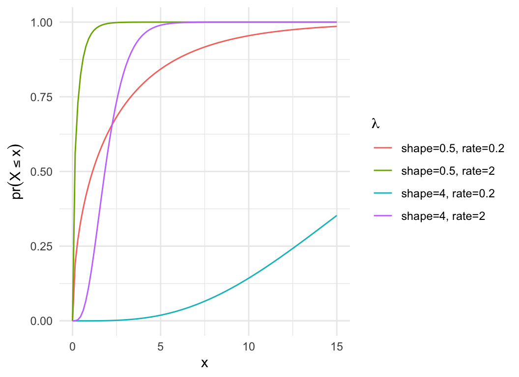
Gamma distribution
- Expenential is a special case of Gamma where shape = 1
- Continuous, defined on \((0,
\infty)\)
- Highly generalised distribution, used in many cases for strictly
positive variables
- Imagine observing a variable \(X\),
such that:
- \(X_i \sim
\mathrm{Poisson}(\lambda_i)\) (i.e., a mixture of Poisson
distribtutions)
- \(\lambda \sim
\mathrm{Gamma}\)
- It follows that \(X \sim \mathrm{Negative
Binomial}\)
dat = expand.grid(x=seq(0,15, length.out=100), shape=c(0.5, 4), rate = c(0.2, 2))
dat$pdf = with(dat, dgamma(x, shape=shape, rate = rate))
dat$cdf = with(dat, pgamma(x, shape=shape, rate = rate))
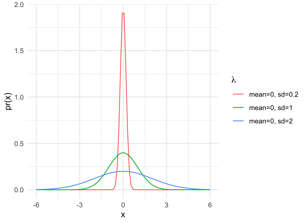
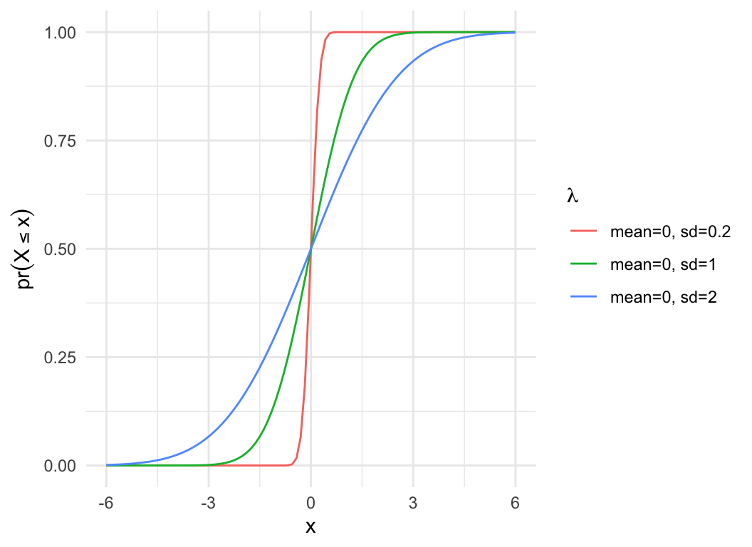
Normal distribution
- Produced by additive processes (log-normal produced by
multiplicative processes)
- Continuous, defined on \((-\infty,
\infty)\)
dat = expand.grid(x=seq(-6,6, length.out=100), mu=0, sd = c(0.2, 1, 2))
dat$pdf = with(dat, dnorm(x, mu, sd))
dat$cdf = with(dat, pnorm(x, mu, sd))
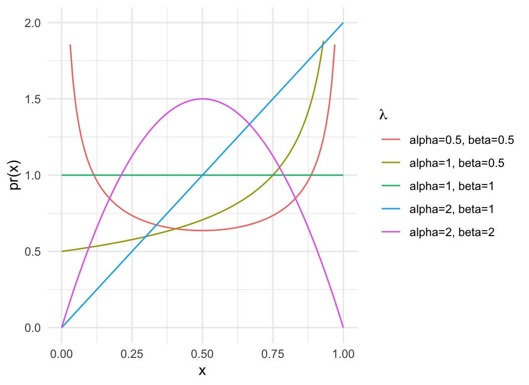
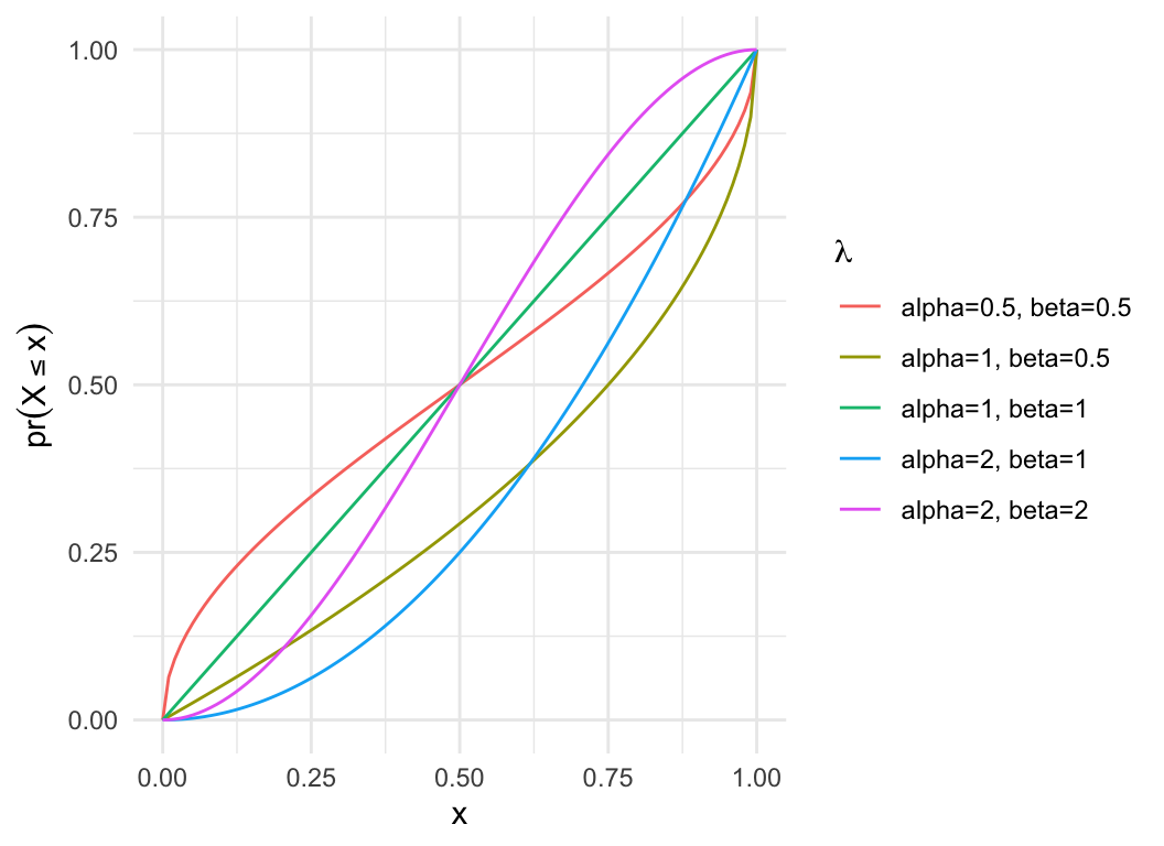
Beta distribution
- Closely related to Binomial; often models the \(p\) parameter for non-stationary
Binomials
- Also used to model proportions
- Continuous, defined on \((0,
1)\)
dat = expand.grid(x=seq(0,1, length.out=100), alpha=c(0.5, 1, 2), beta = c(0.5, 1, 2))
dat$pdf = with(dat, dbeta(x, alpha, beta))
dat$cdf = with(dat, pbeta(x, alpha, beta))
Distribution functions
- A probability density function (PDF) is a function
f(x) that:
- is defined on an interval [a,b] (may be infinite)
- is positive
- is regular—one value of f(x) for every value of (x), and \(\frac{df(x)}{dx}\) is finite
- \(\int_a^b f(x)dx = 1\)
d functions in R (probability density)
– dnorm, dgamma, etc- For discrete distributions, called a probability mass
function (PMF)
- Every PDF/PMF has a CDF
- \(F(x) = \int_a^x f(x)dx\)
- The probability of a value between \(a\) and \(x\)
p functions in R (cumulative
probability) – pnorm, pgamma,
etc