Maximum Likelihood & Optimisation
Adrienne Étard
02.02.2026
The problem of parameter estimation
- In the Zombie example, we knew the probability of being a zombie:
\(p_z = 0.3\)
- We wanted to know the probability of observing some number of
zombies \(k\) in a sample of \(n=10\)
- More typically, we would observe \(k\) via taking a sample of size
\(n\), and then try to estimate \(p_z\).
Sampling a population
- We sampled a large population to determine the rate of zombism.
- Assume samples were random, iid
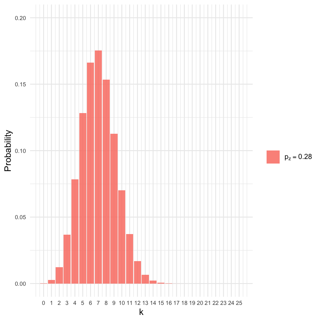
- Given a sample of \(n=25\), we
observed \(k=7\) zombies.
- Estimate \(p_z\), the proportion of
the population that is a zombie.
Sampling a population
- We sampled a large population to determine the rate of zombism.
- Assume samples were random, iid
- Given a sample of \(n=25\), we
observed \(k=7\) zombies.
- Estimate \(p_z\), the proportion of
the population that is a zombie.
- Intuition: We know the best estimate is \(p_z = 7/25 \approx 0.28\). Why?
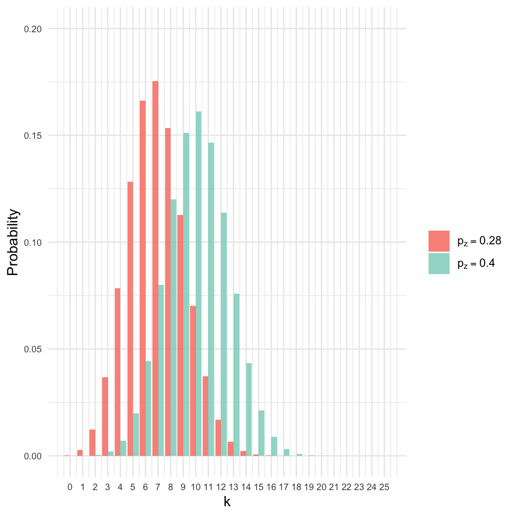
- However: Many other values of \(p_z\) are nearly as likely.
- Here, even if \(p_z = 0.4\), there
is an 8% chance of getting \(k =
7\).
Parameter estimation
- We need a general method for parameter
estimation
- In this case, want to estimate \(p_z\)
- Understanding the uncertainty in our estimate would
also be nice
The likelihood model
- If I have a model \(\theta\)…
- And a dataset \(X\)…
- Can I compute the probability that the data came from this model?
\(pr(X | \theta)\)
The likelihood model
- Example: \(\theta = p_z\), assume
for the moment that \(p_z = 0.4\)
- What is the probability of observing the data (\(k = 7\) with\(n =
25\)) if this model is true?
The likelihood model
- Example: \(\theta = p_z\), assume
for the moment that \(p_z = 0.4\)
- What is the probability of observing the data (\(k = 7\) with\(n =
25\)) if this model is true?
\[
pr(k=7| p_z = 0.4, n = 25) = ?
\]
Any guesses how?
The likelihood model
- We already described this system with a binomial
process
- This is a generative model: we describe the
statistical process (a binomial process with p = 0.4) that produces the
observed data.
- We can evaluate it with built-in functions in R
The likelihood model
- We already described this system with a binomial
process
- This is a generative model: we describe the
statistical process (a binomial process with p = 0.4) that produces the
observed data.
- We can evaluate it with built-in functions in R
# x is observation, in this case, k = 7
# size is n, the number of trials
# prob is the model parameter
dbinom(x = 7, size = 25, prob = 0.4)
## [1] 0.07998648
The likelihood model
# x is observation, in this case, k = 7
# size is n, the number of trials
# prob is the model parameter
dbinom(x = 7, size = 25, prob = 0.4)
## [1] 0.07998648
We can try another model to see if it’s better:
dbinom(x = 7, size = 25, prob = 0.2)
## [1] 0.1108419
The likelihood model
# x is observation, in this case, k = 7
# size is n, the number of trials
# prob is the model parameter
dbinom(x = 7, size = 25, prob = 0.4)
## [1] 0.07998648
We can try another model to see if it’s better:
dbinom(x = 7, size = 25, prob = 0.2)
## [1] 0.1108419
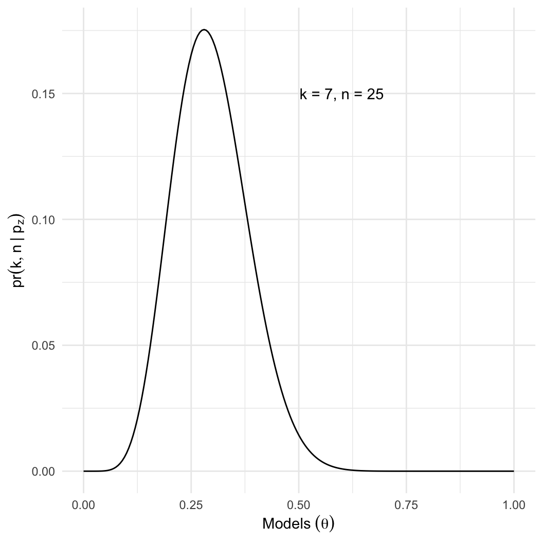
And we can plot it against many different potential models
# different potential values for p, which must be between 0 and 1
models = seq(0, 1, 0.005)
probs = dbinom(x = 7, size = 25, prob = models)
binom_models = data.frame(models, probs)
binom_plot = ggplot(binom_models, aes(x = models, y = probs)) + geom_line()
Likelihood functions
- The likelihood function is a function f of
the data \(X\) and model/parameters
\(\theta\)
- Here \(X = \{k\}\) and \(\theta = \{p_z\}\)
- \(n\) is a constant defined by our
study design.
- \(f(X,\theta)\) returns the
probability of observing \(X\), given a particular model \(\theta\): \(pr(X|\theta)\)
- Here, the binomial PMF is a useful likelihood function
Likelihood functions
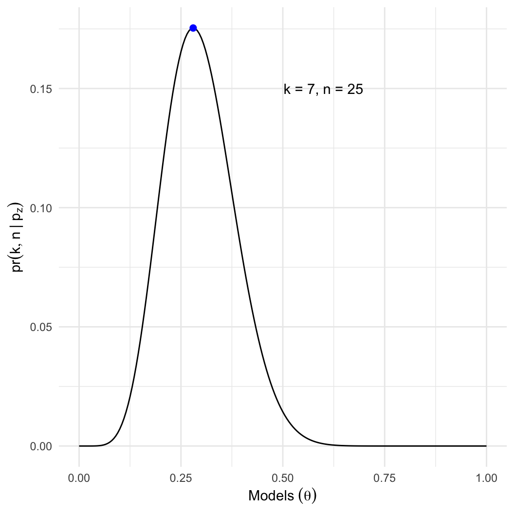
- Intuition is fine, but how do we estimate or solve for the maximum
likelihood? Guessing might take a long time!
Solving for the MLE
\[
\begin{aligned}
\mathcal{L}(k,n|p) & = {n \choose k} p^k(1-p)^{(n-k)}
\end{aligned}
\]
Solving for the MLE
\[
\begin{aligned}
\mathcal{L}(k,n|p) & = {n \choose k} p^k(1-p)^{(n-k)} \\
\frac{d \mathcal{L}(k,n|p)}{dp} & = {n \choose
k}kp^{k-1}(1-p)^{(n-k)} - {n \choose k} p^k (n-k)(1-p)^{(n-k-1)}
\end{aligned}
\]
Solving for the MLE
\[
\begin{aligned}
\mathcal{L}(k,n|p) & = {n \choose k} p^k(1-p)^{(n-k)} \\
\frac{d \mathcal{L}(k,n|p)}{dp} & = {n \choose
k}kp^{k-1}(1-p)^{(n-k)} - {n \choose k} p^k (n-k)(1-p)^{(n-k-1)} \\
& = 0
\end{aligned}
\]
Solving for the MLE
\[
\begin{aligned}
\frac{d \mathcal{L}(k,n|p)}{dp} = 0 & = {n \choose
k}kp^{k-1}(1-p)^{(n-k)} - {n \choose k} p^k (n-k)(1-p)^{(n-k-1)} \\
{n \choose k} p^k (n-k)(1-p)^{(n-k-1)} & = {n \choose
k}kp^{k-1}(1-p)^{(n-k)}
\end{aligned}
\]
Solving for the MLE
\[
\begin{aligned}
\frac{d \mathcal{L}(k,n|p)}{dp} = 0 & = {n \choose
k}kp^{k-1}(1-p)^{(n-k)} - {n \choose k} p^k (n-k)(1-p)^{(n-k-1)} \\
{\xcancel{n \choose k}} p^k (n-k)(1-p)^{(n-k-1)} & = {\xcancel{n
\choose k}}kp^{k-1}(1-p)^{(n-k)}
\end{aligned}
\]
Solving for the MLE
\[
\begin{aligned}
\frac{d \mathcal{L}(k,n|p)}{dp} = 0 & = {n \choose
k}kp^{k-1}(1-p)^{(n-k)} - {n \choose k} p^k (n-k)(1-p)^{(n-k-1)} \\
{n \choose k} p^k (n-k)(1-p)^{(n-k-1)} & = {n \choose
k}kp^{k-1}(1-p)^{(n-k)}
\\
p(p^{k-1}) (n-k)(1-p)^{(n-k-1)} & = kp^{k-1}(1-p)(1-p)^{(n-k-1)} \\
\end{aligned}
\]
Solving for the MLE
\[
\begin{aligned}
\frac{d \mathcal{L}(k,n|p)}{dp} = 0 & = {n \choose
k}kp^{k-1}(1-p)^{(n-k)} - {n \choose k} p^k (n-k)(1-p)^{(n-k-1)} \\
{n \choose k} p^k (n-k)(1-p)^{(n-k-1)} & = {n \choose
k}kp^{k-1}(1-p)^{(n-k)}
\\
p{\xcancel{(p^{k-1})}} (n-k){\xcancel{(1-p)^{(n-k-1)}}} & =
k{\xcancel{p^{k-1}}}(1-p){\xcancel{(1-p)^{(n-k-1)}}} \\
\end{aligned}
\]
Solving for the MLE
\[
\begin{aligned}
\frac{d \mathcal{L}(k,n|p)}{dp} = 0 & = {n \choose
k}kp^{k-1}(1-p)^{(n-k)} - {n \choose k} p^k (n-k)(1-p)^{(n-k-1)} \\
{n \choose k} p^k (n-k)(1-p)^{(n-k-1)} & = {n \choose
k}kp^{k-1}(1-p)^{(n-k)}
\\
p(p^{k-1}) (n-k)(1-p)^{(n-k-1)} & = kp^{k-1}(1-p)(1-p)^{(n-k-1)} \\
p (n-k) & = k(1-p) \\
pn -pk & = k-pk \\
\end{aligned}
\]
Solving for the MLE
\[
\begin{aligned}
\frac{d \mathcal{L}(k,n|p)}{dp} = 0 & = {n \choose
k}kp^{k-1}(1-p)^{(n-k)} - {n \choose k} p^k (n-k)(1-p)^{(n-k-1)} \\
{n \choose k} p^k (n-k)(1-p)^{(n-k-1)} & = {n \choose
k}kp^{k-1}(1-p)^{(n-k)}
\\
p(p^{k-1}) (n-k)(1-p)^{(n-k-1)} & = kp^{k-1}(1-p)(1-p)^{(n-k-1)} \\
p (n-k) & = k(1-p) \\
pn - {\xcancel{pk}} & = k-{\xcancel{pk}} \\
\end{aligned}
\]
Solving for the MLE
\[
\begin{aligned}
\frac{d \mathcal{L}(k,n|p)}{dp} = 0 & = {n \choose
k}kp^{k-1}(1-p)^{(n-k)} - {n \choose k} p^k (n-k)(1-p)^{(n-k-1)} \\
{n \choose k} p^k (n-k)(1-p)^{(n-k-1)} & = {n \choose
k}kp^{k-1}(1-p)^{(n-k)}
\\
p(p^{k-1}) (n-k)(1-p)^{(n-k-1)} & = kp^{k-1}(1-p)(1-p)^{(n-k-1)} \\
p (n-k) & = k(1-p) \\
pn -pk & = k-pk \\
pn & = k \\
p & = \frac{k}{n} \\
\end{aligned}
\]
Optimisation
- In many (most) cases, analytical solutions are unavailable or
impractical.
- We turn to various algorithms for numerical optimisation
Optimisation
- In many (most) cases, analytical solutions are unavailable or
impractical.
- We turn to various algorithms for numerical optimisation
# define our data set
n = 25
k = 7

# write a custom function that returns the log likelihood
llfun = function(p, n, k) {
  dbinom(k, n, p, log=TRUE) ## why log??
}

# we need an initial guess for the parameter we want to optimise
p_init = 0.5
Optimisation
- In many (most) cases, analytical solutions are unavailable or
impractical.
- We turn to various algorithms for numerical optimisation
# optim will start at p_init, evaluate llfun using the data we pass
# and return the optimum (if found)
# the terms n = ... and k = ... must be named the way they are in llfun
optim(p_init, llfun, method = "Brent", n = n, k = k, control = list(fnscale = -1), lower=0, upper=1)
## $par
## [1] 0.28
##
## $value
## [1] -1.740834
##
## $counts
## function gradient
##       NA       NA
##
## $convergence
## [1] 0
##
## $message
## NULL
Parameter estimation in Stan
- Stan is a modelling language for scientific computing
- We use probabilistic programming
- deterministic variables:
a = b * c
- Stochastic variables:
y ~ normal(mu, sigma)
Workflow
- Write a Stan model in a
.stan file
- Prepare all data in R
- Use the
rstan package to invoke the Stan interpreter
- Translates your model into a C++ program then compiles for your
computer
- Run the program from R using functions in the
rstan
package.
Parameter estimation in Stan
- All Stan programs need a
data block where you define
any input data for your model
- Variables must have a type
- Here,
int indicates a variable that is an integer
- Constraints give rules about variables; here k must
be positive, and n >= k
- The data block is also a great place for constants
(like n)!
File: vu_advstats_students/stan/zomb_p.stan
data {
    int <lower = 0> k;
    int <lower = k> n;
}
Parameter estimation in Stan
- In the
parameters block, we define
unknowns that we want to estimate
p is a real number between 0 and 1
File: vu_advstats_students/stan/zomb_p.stan
data {
    int <lower = 0> k;
    int <lower = k> n;
}
parameters {
    real <lower = 0, upper = 1> p;
}
Parameter estimation in Stan
- In the
model block we specify our likelihood function
k comes from a binomial distribution with n
observations and probability parameter p
File: vu_advstats_students/stan/zomb_p.stan
data {
    int <lower = 0> k;
    int <lower = k> n;
}
parameters {
    real <lower = 0, upper = 1> p;
}
model {
    k ~ binomial(n, p);
}
Parameter estimation in Stan
- In R, we load the
rstan package
- Next we compile the model using
stan_model
- Compiled models don’t need to be re-compiled unless the code in the
.stan file changes!
# assuming working directory is vu_advstats_students
library(rstan)
zomb_p = stan_model("stan/zomb_p.stan")
Parameter estimation in Stan
- We next create a data list that we will pass on to Stan
- Finally, we can use
optimizing, which works similar to
optim but for Stan models
# assuming working directory is vu_advstats_students
library(rstan)

## reminder: only do this once unless zomb_p.stan changes!
zomb_p = stan_model("stan/zomb_p.stan")


# prepare data
# names must match the data block in Stan
zomb_data = list(n = 25, k = 7)

# estimate the parameter
optimizing(zomb_p, data = zomb_data)
## $par
##         p
## 0.2800145
##
## $value
## [1] -14.82383
##
## $return_code
## [1] 0
##
## $theta_tilde
##              p
## [1,] 0.2800145
Generalising to multiple observations
- Remember the product rule: for two independent events,
\[pr(A,B) = pr(A)pr(B)\]
- Likelihoods are probabilities, and we like to assume each data point
is independent. Thus:
\[
\begin{array}
\mathcal{L}(X_{1..n}|\theta) & = \prod_{i=1}^{n}
\mathcal{L}(X_i|\theta) \\
& \mathrm{or} \\
\log \mathcal{L}(X_{1..n}|\theta) &= \sum_{i=1}^{n} \log
\mathcal{L}(X_i|\theta)
\end{array}
\]
# define our data set and initial guess
n_vec = c(25, 12, 134)
k_vec = c(7, 4, 27)
p_init = 0.5

# we take the sum of all the individual log liklihoods
llfun = function(p, n, k) {
  sum(dbinom(k, n, p, log=TRUE))
}

# take only the part we want out of this, $par, the parameter estimate
optim(p_init, llfun, method = "Brent", n = n_vec, k = k_vec,
      control = list(fnscale = -1), lower=0, upper=1)$par
## [1] 0.2222222
Multiple observations in Stan
k and n are arrays of
ints, each with a length of n_obs- Comments indicated with
//
- The
binomial function is vectorised, can operate on
multiple observations with no changes.
data {
    int <lower = 1> n_obs; // number of data points
    array [n_obs] int <lower = 0> k;
    array [n_obs] int <lower = 0> n; // number of trials for each data point
}
parameters {
    real <lower = 0, upper = 1> p;
}
model {
    k ~ binomial(n, p);
}
zomb_p2 = stan_model("stan/zomb_p2.stan")
Multiple observations in Stan
# prepare data
# names must match the data block in Stan
zomb_data = list(n = c(25, 12, 134), k = c(7, 4, 27), n_obs = 3)

# estimate the parameter
optimizing(zomb_p2, data = zomb_data)$par
##         p
## 0.2222237
Why Bayes?
- I want to describe some phenomenon (“model”; \(\theta\))
- I have some general (“prior”) knowledge about the question: \(pr(\theta)\)
- I gather additional information (“data”; \(X\))
What is the probability that my model is correct given what I already
know about it and what I’ve learned?
\[ pr(\theta | X) \]
Applying Bayes’ Theorem
- We already know an expression for this:
\[
pr(\theta | X) = \frac{pr(X|\theta)pr(\theta)}{pr(X)}
\]
Applying Bayes’ Theorem
- We already know an expression for this:
\[
pr(\theta | X) = \frac{pr(X|\theta)pr(\theta)}{pr(X)}
\]
- The goal, \(pr(\theta | X)\), is
called the posterior probability of \(\theta\)
- We have already seen \(pr(X|\theta)\); this is the
likelihood of the data
- \(pr(\theta)\) is often called the
prior probability of \(\theta\). Could also be called
“other information about \(\theta\)”
- What about \(pr(X)\)? This is the
normalizing constant
When we do Bayesian inference, each of these terms is a full
probability distribution
The normalizing constant
- For the first zombie problem, we had a single observation (“I tested
positive”), we were able to add up all of the ways one could test
positive.
- \(pr(T) = pr(T,Z) + pr(T,Z') =
pr(T|Z)pr(Z) + pr(T|Z')pr(Z')\)
The normalizing constant
- For the first zombie problem, we had a single observation (“I tested
positive”), we were able to add up all of the ways one could test
positive.
- \(pr(T) = pr(T,Z) + pr(T,Z') =
pr(T|Z)pr(Z) + pr(T|Z')pr(Z')\)
More generally:
- \(pr(X) = \sum_i^n
pr(X|\theta_i)pr(\theta_i)\) where all possible models are in the
set \(n\)
- What about for continuous problems?
- There are an infinite number of possible models if \(pr(\theta)\) is a continuous PDF.
- There are infinitely many possible datasets if X is real-valued
\[
pr(X) = \int_a^b pr(X|\theta)pr(\theta)d \theta
\]
- This integral can be challenging to compute
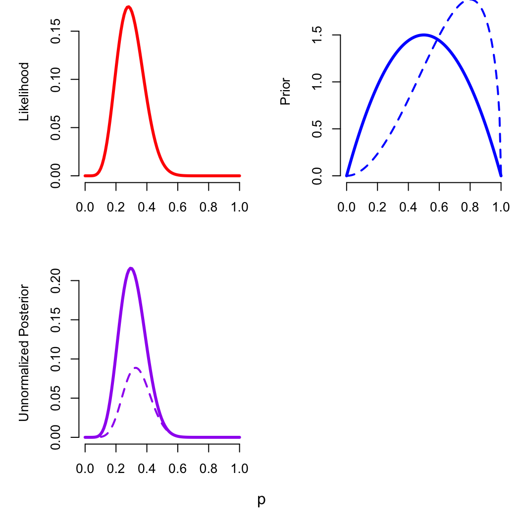
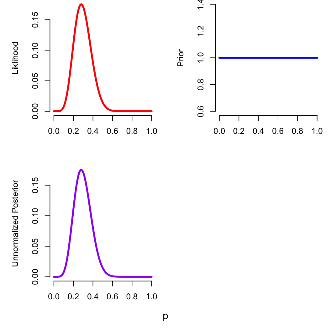
Proportional Bayes’ Theorem
- \(pr(X)\) is a constant;
it adjusts the height of the distribution so that the posterior
integrates to 1
- If all we want to do is estimate the maximum value, we can safely
ignore it
Proportional Bayes’ Theorem
- \(pr(X)\) is a constant;
it adjusts the height of the distribution so that the posterior
integrates to 1
- If all we want to do is estimate the maximum value, we can safely
ignore it
\[
pr(\theta|X) \propto pr(X|\theta)pr(\theta)
\]
- For our example, we used the binomial PMF for the likelihood:
\[
pr(X|\theta) = pr(k,n|p) = {n \choose k} p^k(1-p)^{(n-k)}
\]
How to choose the prior, \(pr(\theta)\)?
What do we know about p?
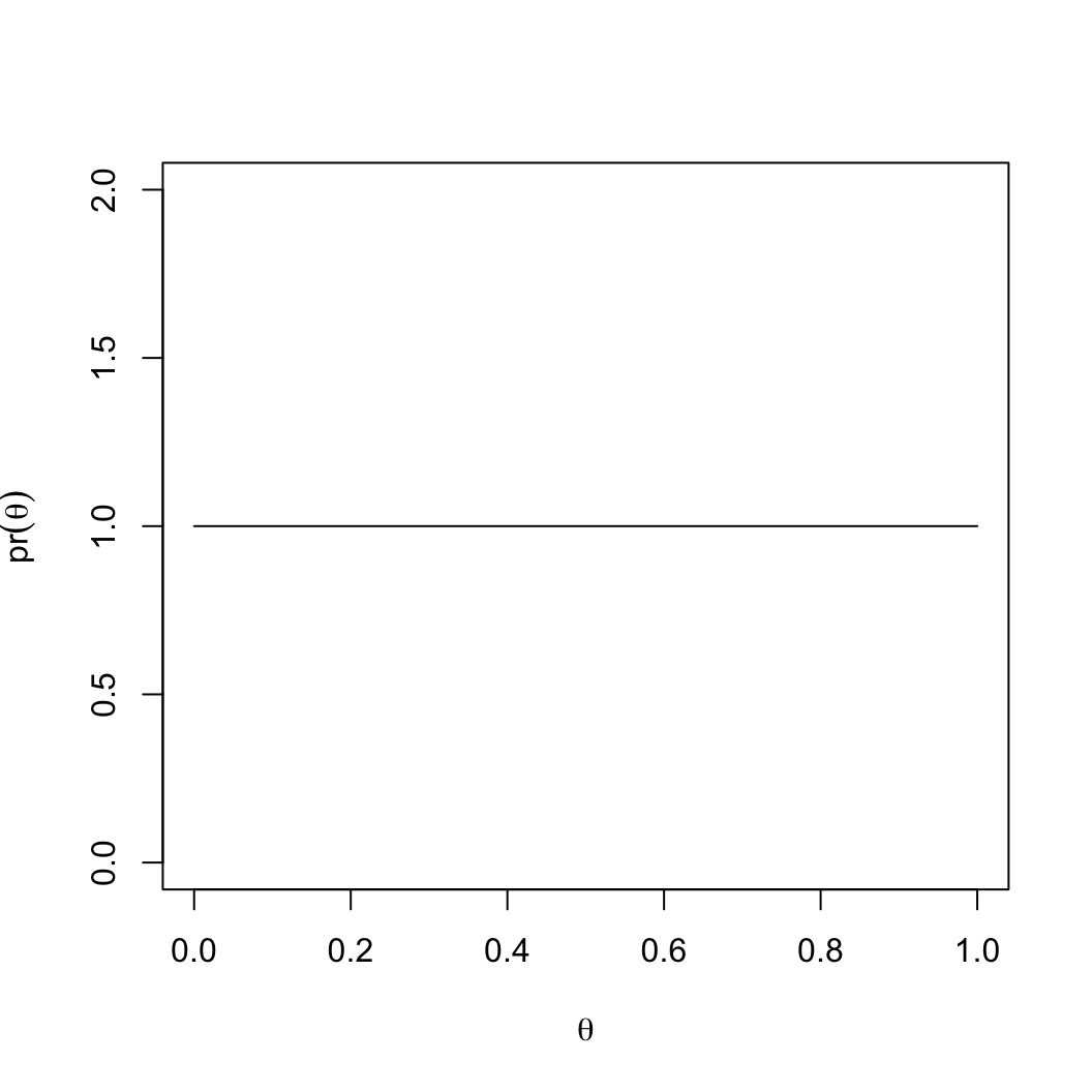
- Must be between 0 and 1.
- We could assign equal probabilities using a uniform
distribution:
theta = seq(0, 1, 0.01)
pr_theta = dunif(theta, min = 0, max = 1)
plot(theta, pr_theta, type = 'l')
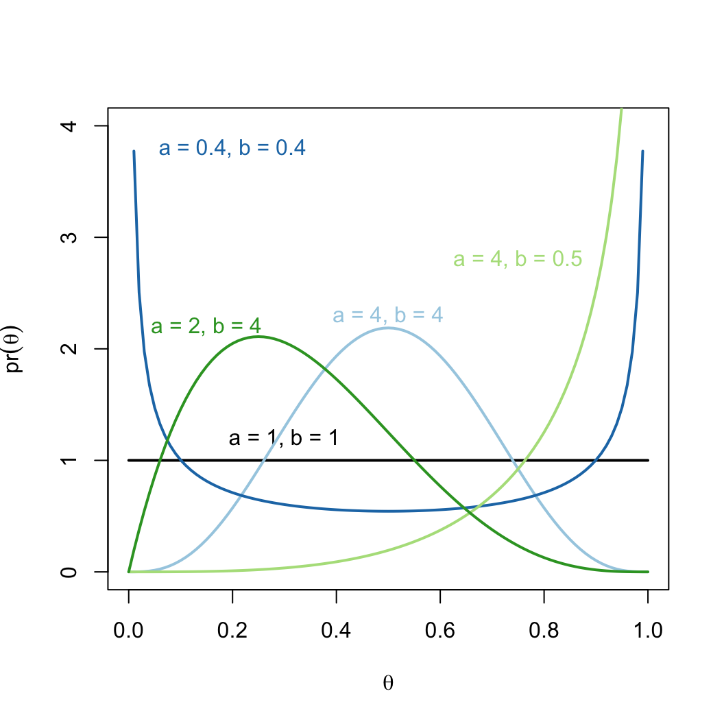
What do we know about p?
- Must be between 0 and 1.
- We could assign equal probabilities using a uniform
distribution.
- Not very flexible. Maybe we think central values are slightly more
likely?
- A beta distribution makes many shapes possible
theta = seq(0, 1, 0.01)
pr_theta_1 = dbeta(theta, shape1 = 1, shape2 = 1)
Maximum A Posteriori Estimation
- If we just want a Bayesian point estimate for \(\theta\), we can use the same algorithms
for MLE
- This is know as the maximum a posteriori (MAP)
estimate, Bayesian equivalent to the MLE
- We ignore the normalising constant and incorporate a prior into the
methods we used before
log_liklihood = function(p, n, k)
  sum(dbinom(k, n, p, log=TRUE))

log_prior = function(p, a, b)
  dbeta(p, a, b, log = TRUE)

log_posterior = function(p, n, k, a, b)
  log_liklihood(p, n, k) + log_prior(p, a, b)
// Saved in vu_advstats_students/stan/zomb_p_bayes.stan
data {
    int <lower = 1> n_obs;
    array [n_obs] int <lower = 0> k;
    array [n_obs]int <lower = 0> n;
    real <lower = 0> a;
    real <lower = 0> b;
}
parameters {
    real <lower = 0, upper = 1> p;
}
model {
    k ~ binomial(n, p);
    p ~ beta(a, b);
}
Maximum A Posteriori Estimation
Now we can fit the model, either in R or in Stan
zomb_p_bayes = stan_model("stan/zomb_p_bayes.stan")
zomb_data = list(
    n_obs = 1,
    n = as.array(25), # force a single-value array, avoids an error
    k = as.array(7),
    a = 1, # totally flat prior to start
    b = 1
)

## starting value for the optimisation
p_init = 0.5

optim(p_init, log_posterior, method = "Brent", n = zomb_data$n,
    k = zomb_data$k, a = zomb_data$a, b = zomb_data$b,
    control = list(fnscale = -1), lower=0, upper=1)$par
## [1] 0.28

optimizing(zomb_p_bayes, data = zomb_data)$par
##    p
## 0.28
This prior has no influence on the posterior
Changing the prior
zomb_data$a = 2; zomb_data$b = 2
optimizing(zomb_p_bayes, data = zomb_data)$par
##         p
## 0.2962964
zomb_data$a = 3; zomb_data$b = 1.5
optimizing(zomb_p_bayes, data = zomb_data)$par
##         p
## 0.3272733
These priors are informative, but relatively weak (our data has
weight equivalent to alpha=7, beta=18)
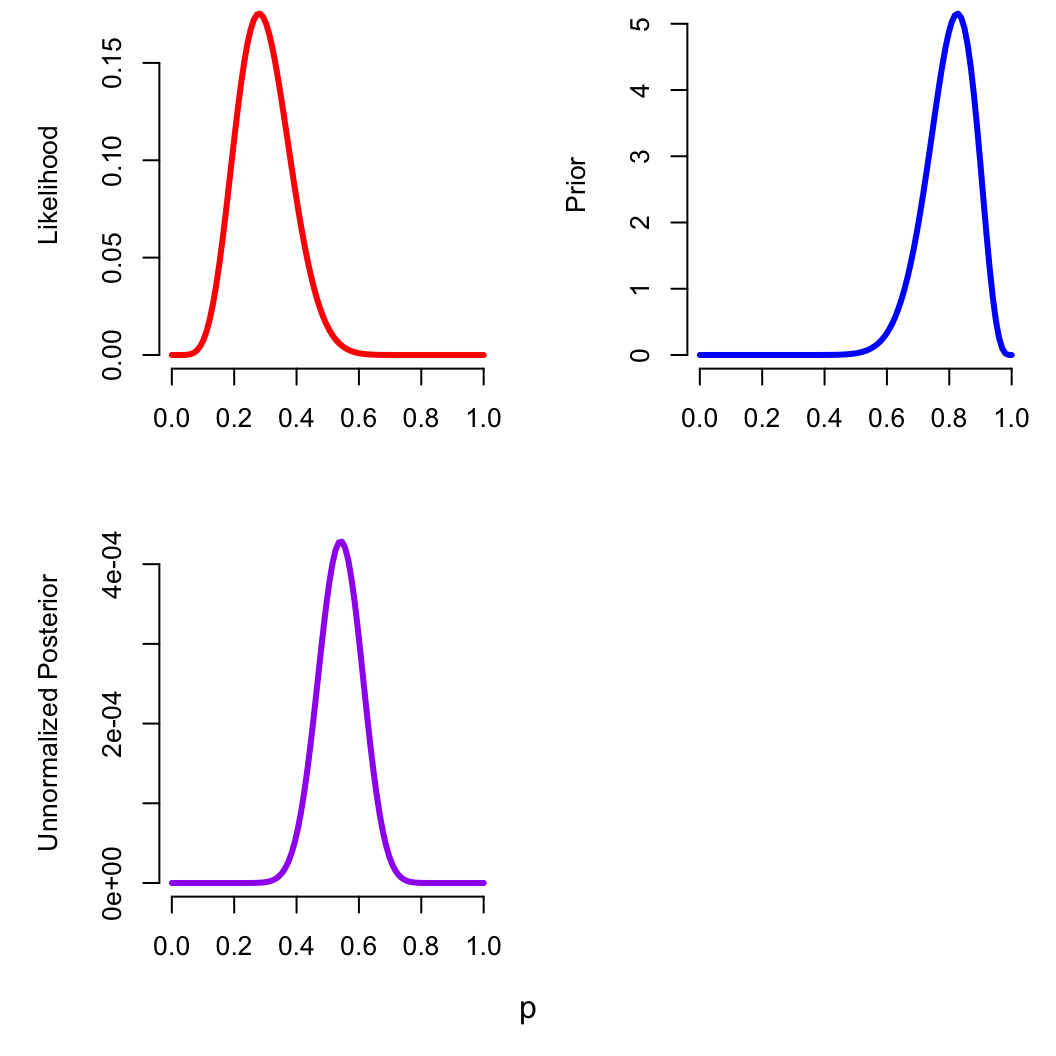
Changing the prior
What if we had already conducted an identical prior sample, with 20
zombies and 5 normals?
zomb_data$a = 20; zomb_data$b = 5
optimizing(zomb_p_bayes, data = zomb_data)$par
##         p
## 0.5416663
Geting a normalized posterior
- We often want to know the full posterior distribution
- For some problems, we have analytical solutions to \(\int pr(X|\theta)pr(\theta)d \theta\)
Geting a normalized posterior
- We often want to know the full posterior distribution
- For some problems, we have analytical solutions to \(\int pr(X|\theta)pr(\theta)d \theta\)
- For the beta-binomial, if:
\[
\begin{aligned}
\overset{\small \color{blue}{prior}}{pr(p)} & = \mathrm{Beta}(a, b)
\\ \\
\overset{\small \color{blue}{likelihood}}{pr(k,n | p)} & =
\mathrm{Binomial}(k, n, p)
\end{aligned}
\]
Geting a normalized posterior
- We often want to know the full posterior distribution
- For some problems, we have analytical solutions to \(\int pr(X|\theta)pr(\theta)d \theta\)
- For the beta-binomial, if:
\[
\begin{aligned}
\overset{\small \color{blue}{prior}}{pr(p)} & = \mathrm{Beta}(a, b)
\\ \\
\overset{\small \color{blue}{likelihood}}{pr(k,n | p)} & =
\mathrm{Binomial}(k, n, p) \\ \\
\overset{\small \color{blue}{posterior}}{pr(p | k,n,a,b)} &=
\mathrm{Beta}(a + k, b + n - k)
\end{aligned}
\]
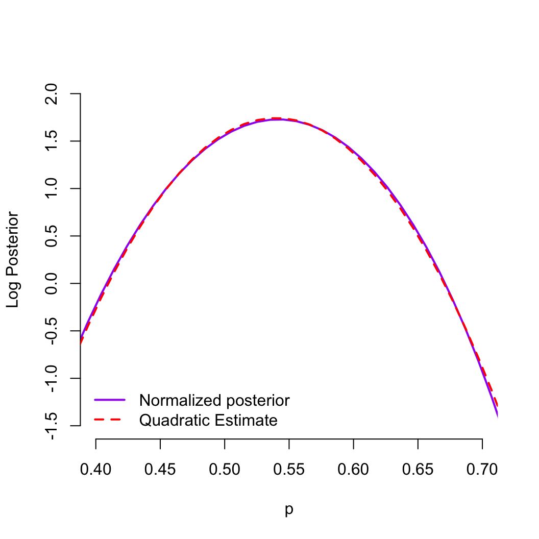
Geting a normalized posterior
- We often want to know the full posterior distribution
- For some problems, we have analytical solutions to \(\int pr(X|\theta)pr(\theta)d \theta\)
- In many cases, the shape of the log posterior is appoximately
quadratic (the posterior is approximately normal)
- Laplace approximation (or Quadratic approximation)
is a method for approximating the shape of this curve
- When the above are unavailable, we can use simulations (e.g.,
MCMC)