The German Tank Problem
Knowns:
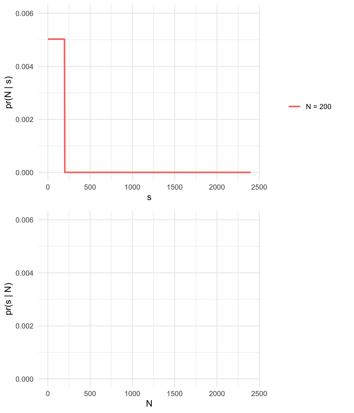
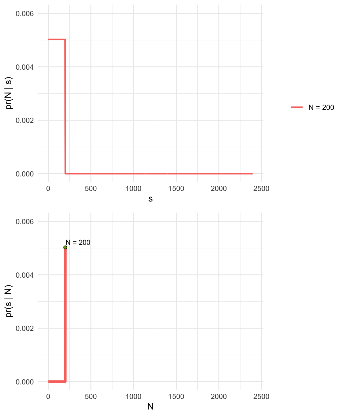
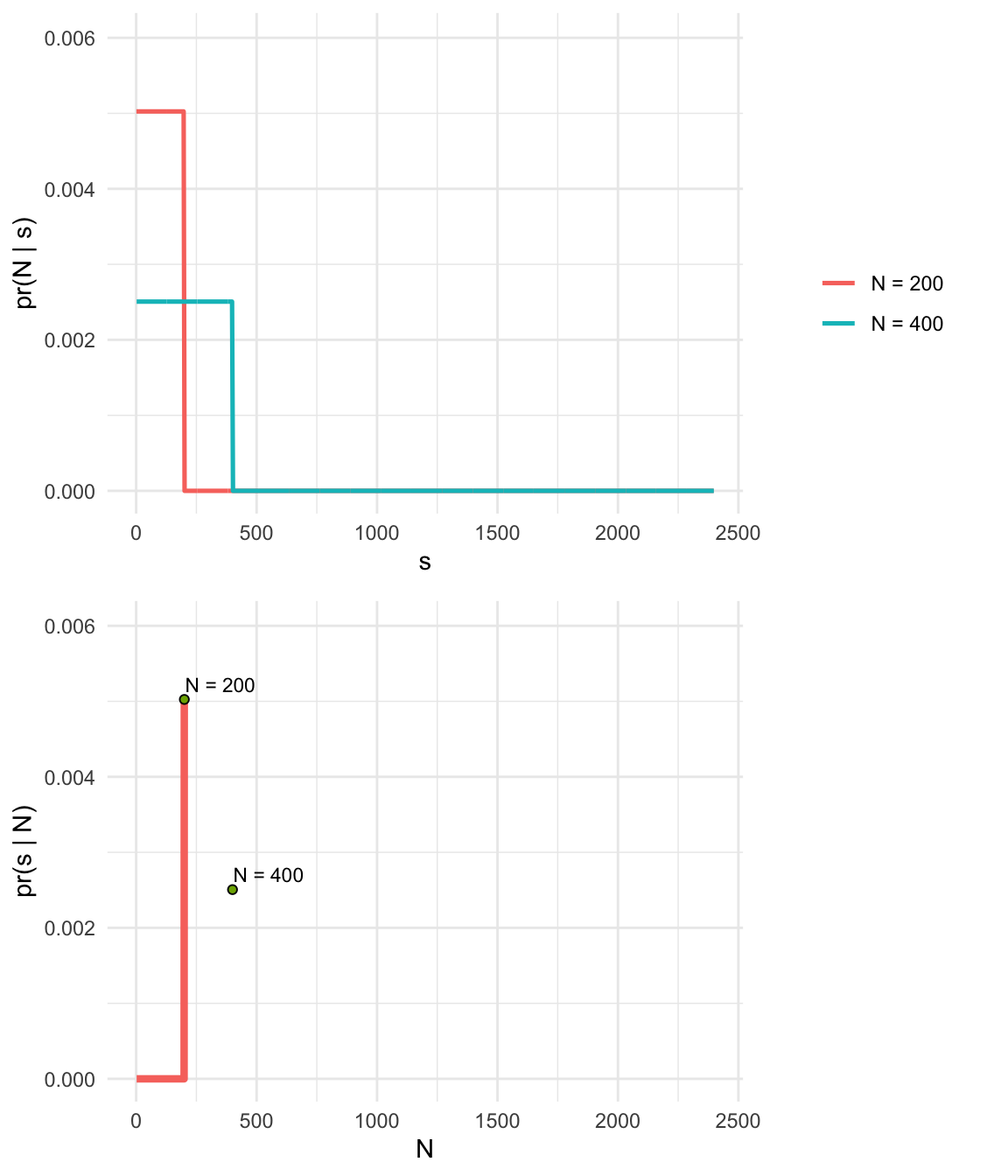
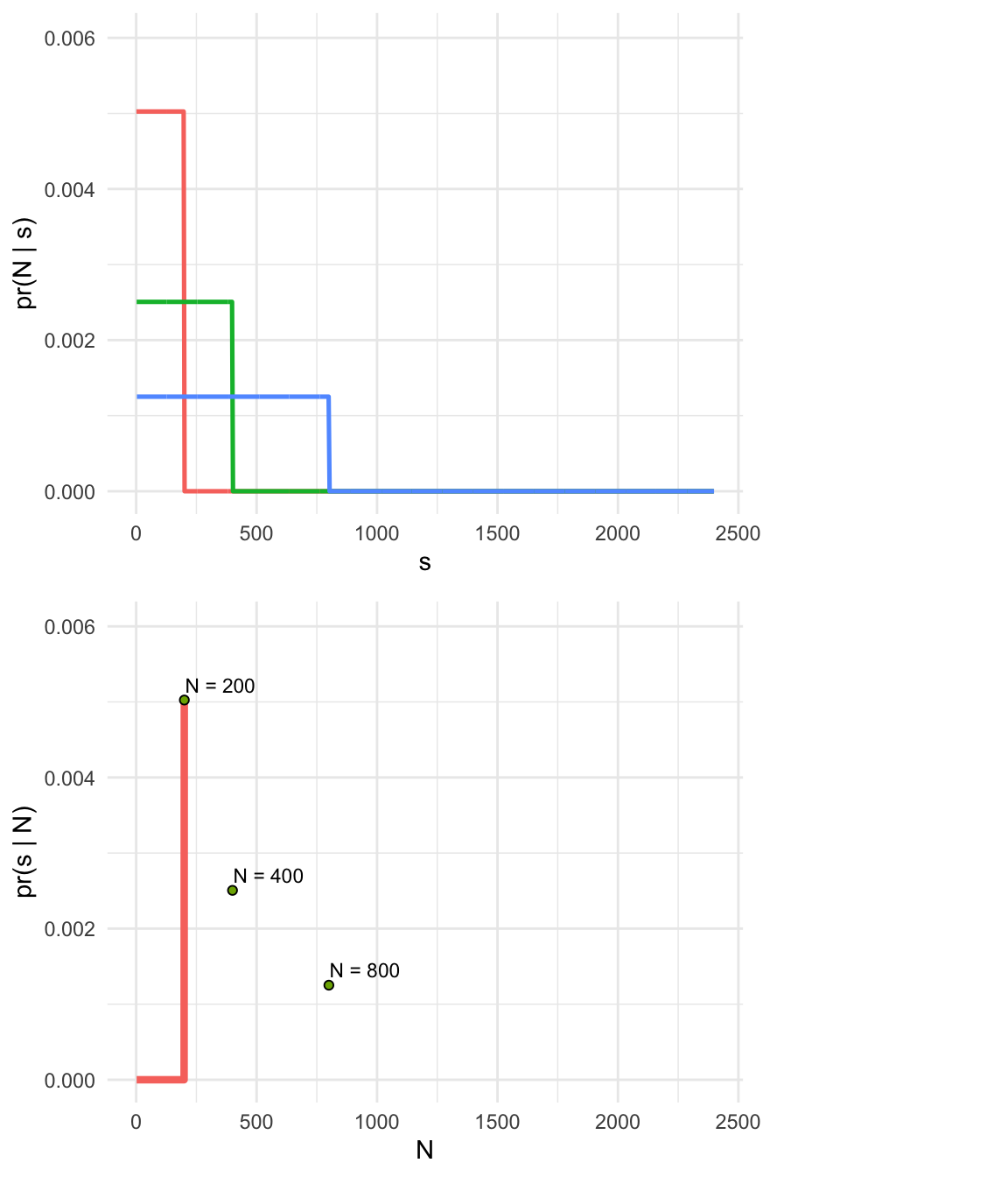
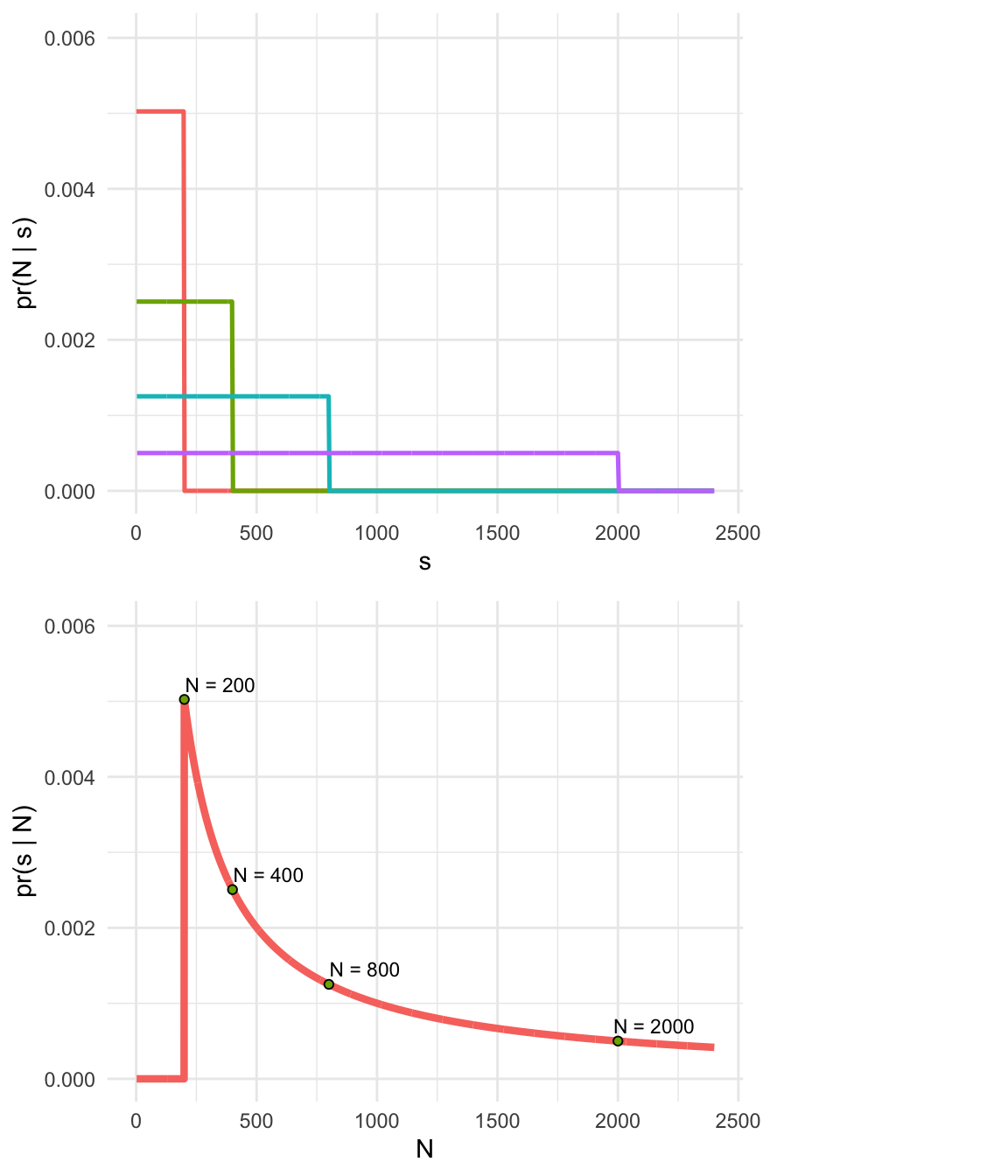
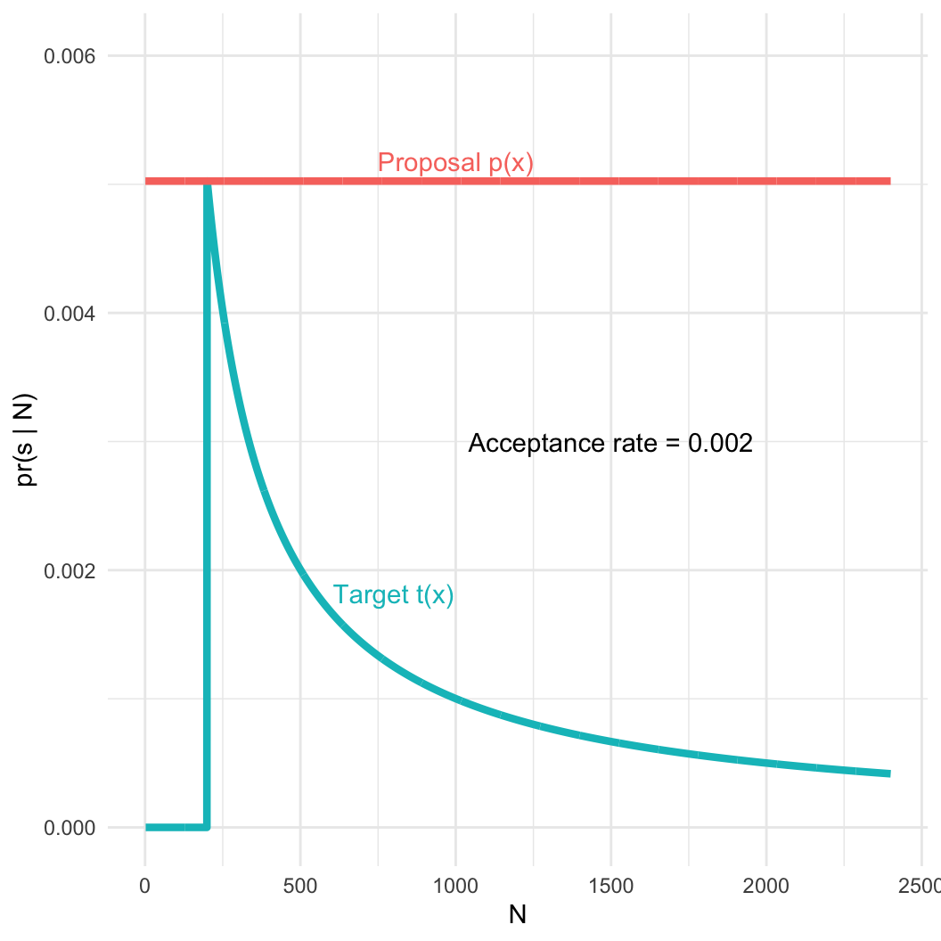
- Captured serial number \(s = 200\)
- Number of tanks \(N >= s\)
- Assume tanks are captured completely at random, so all tanks have the same probability of capture
- This sounds like a uniform distribution!
- Minimum of the distribution is 1, the maximum will be N.
- Hypothesis: We got the biggest tank; \(s = N\)