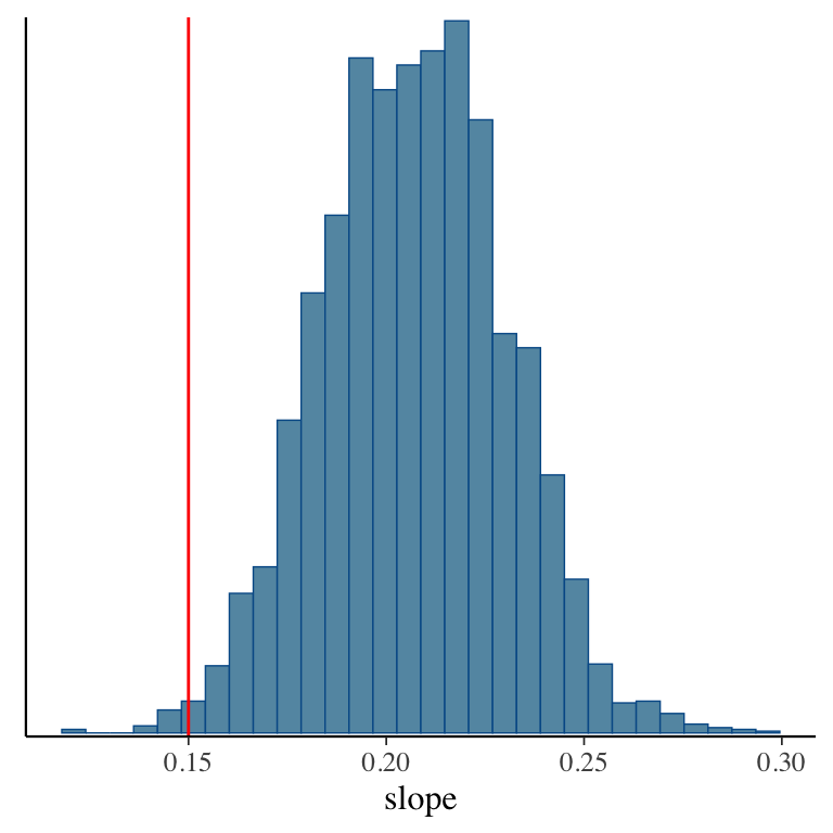
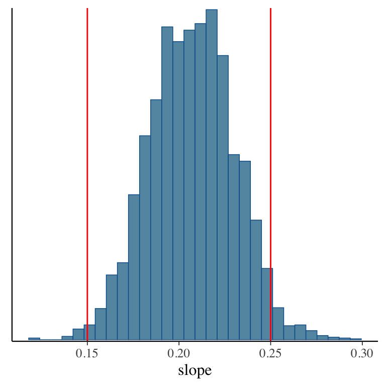
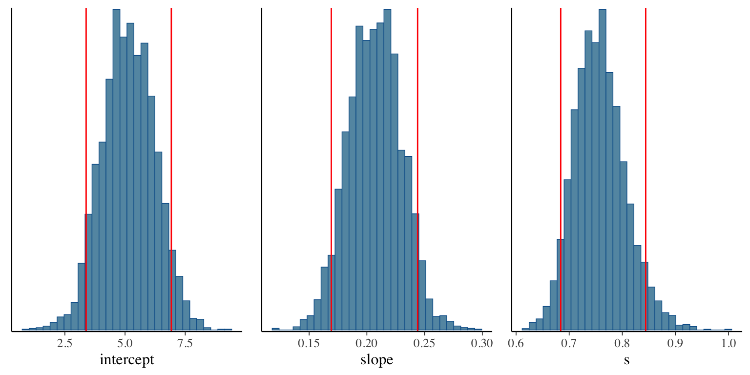
Posterior inference I: Sampling
- Taking samples turns out to be a very useful way to learn about a distribution!
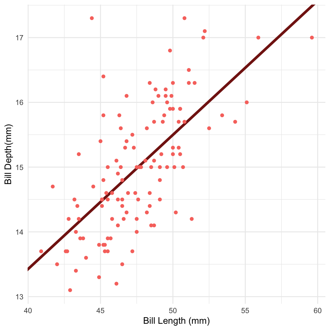
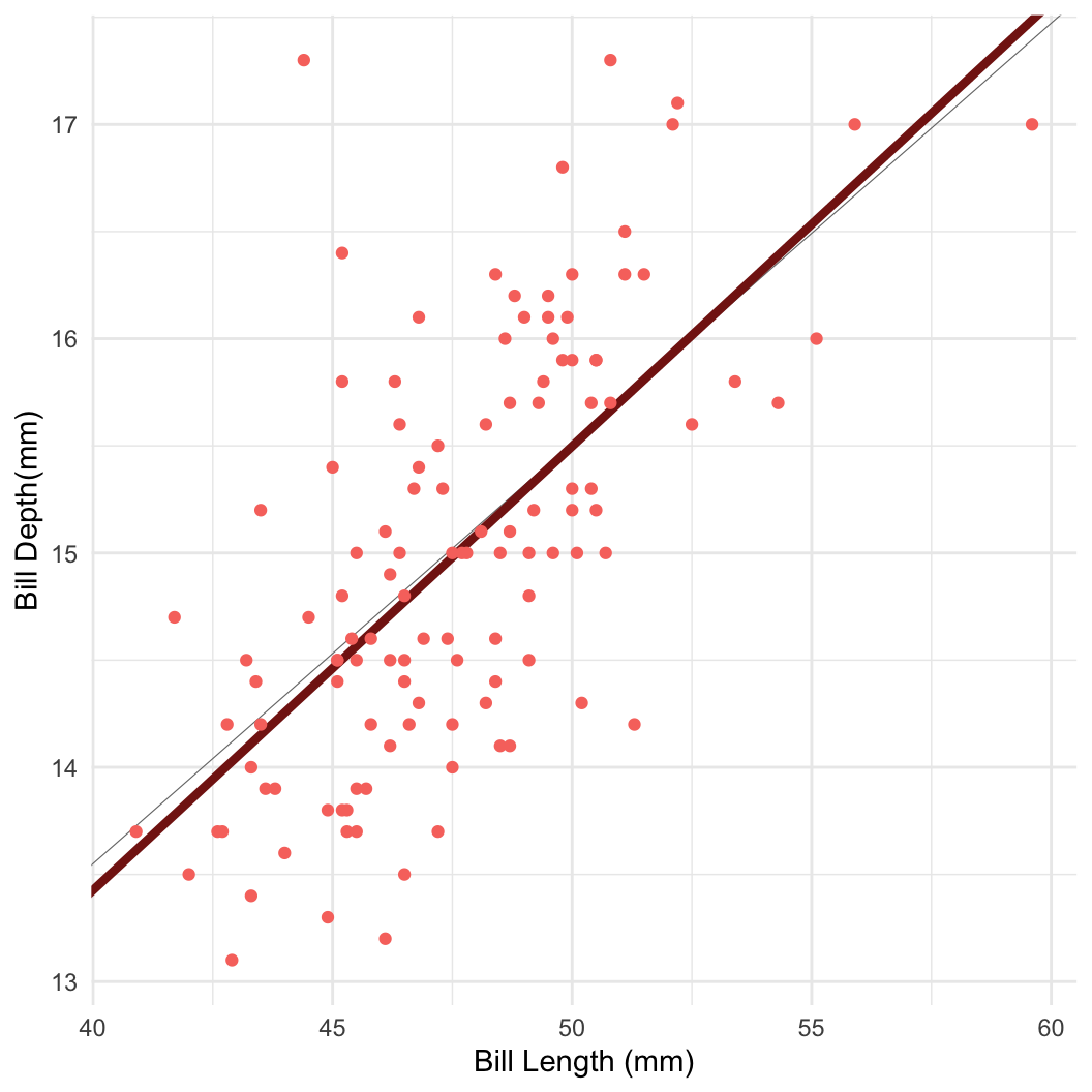
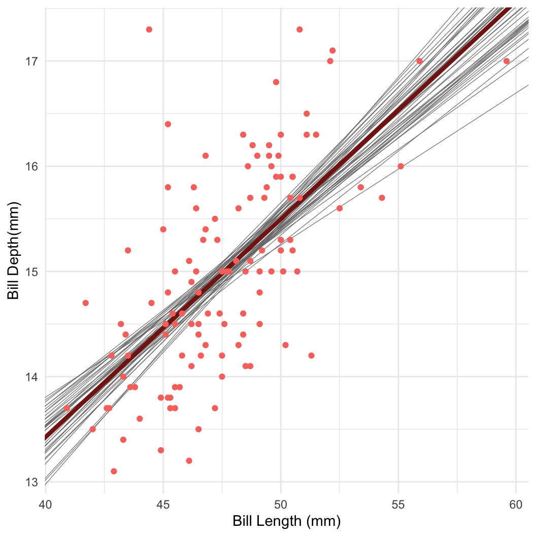
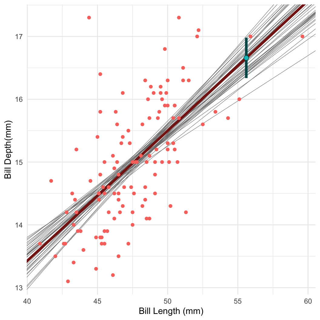
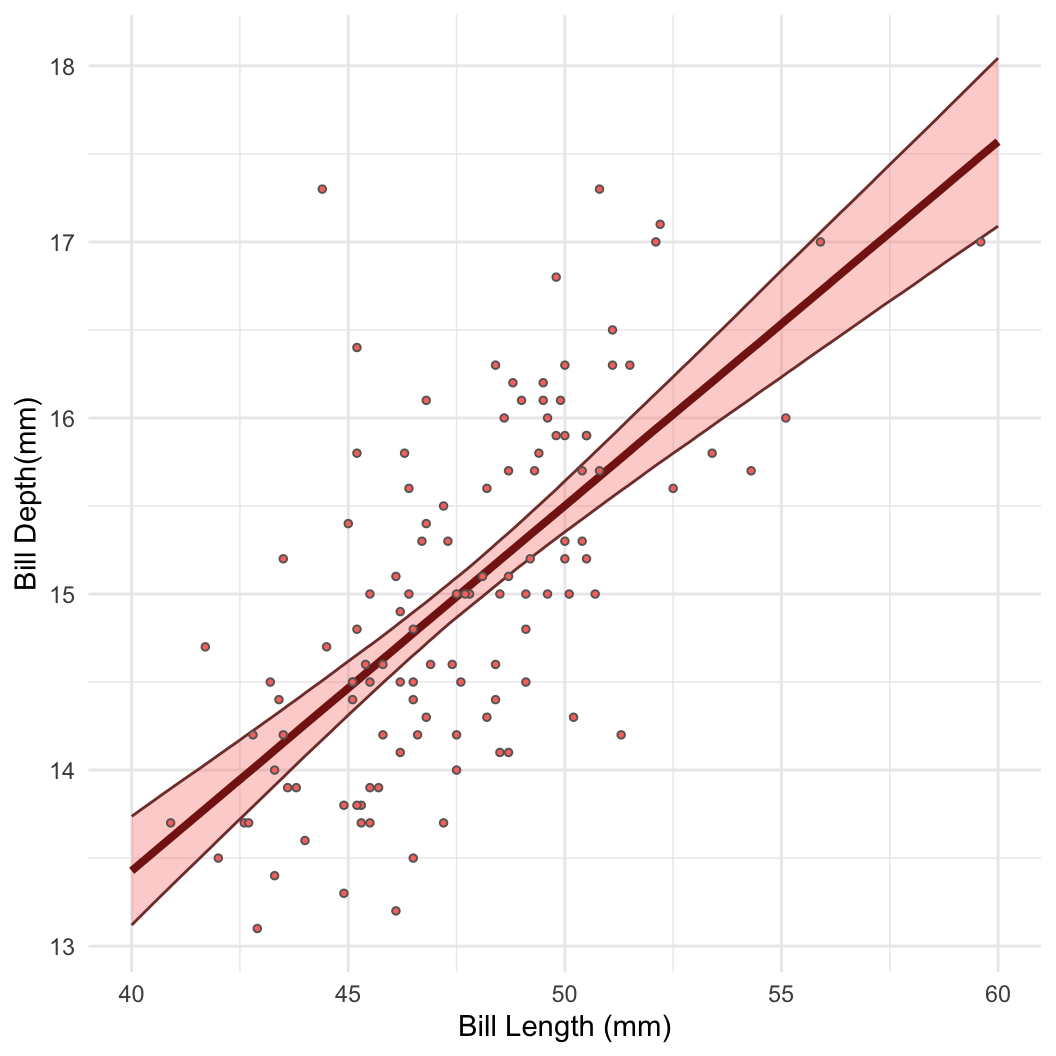
- For example: Bayesian linear regression in Stan
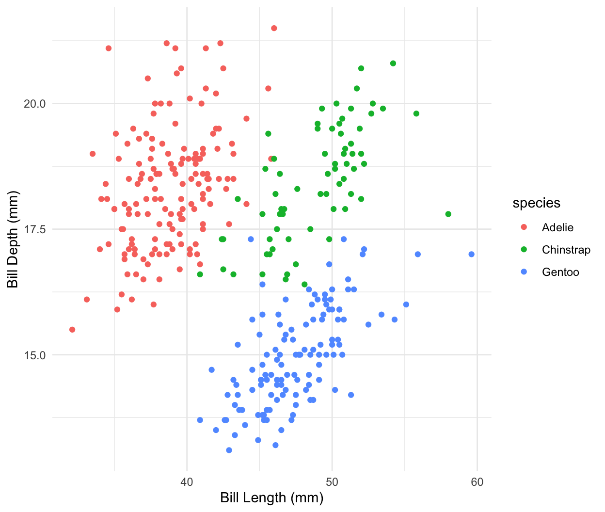
Dataset: Palmer penguins

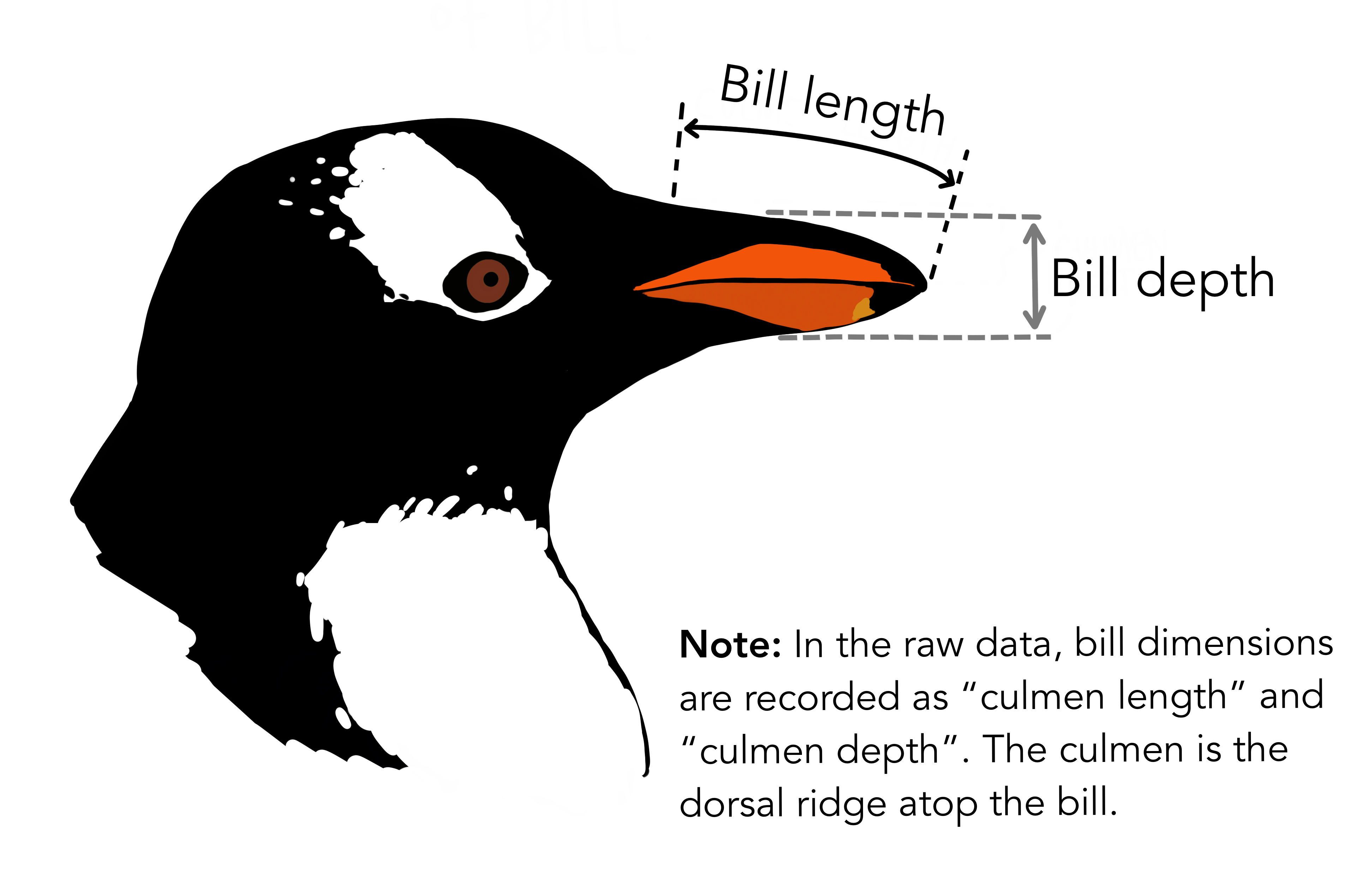
Dataset: Dr. Kristen Gorman, University of Alaska (Gorman et al 2014)
R package
palmerpenguinsArtwork by @allison_horst