Regression problems
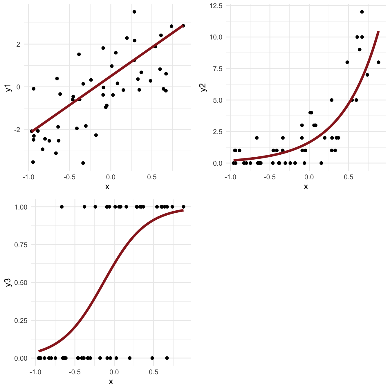
- Many applied problems take the form of a set of observations \(y\) along with one or more covariates \(x\)
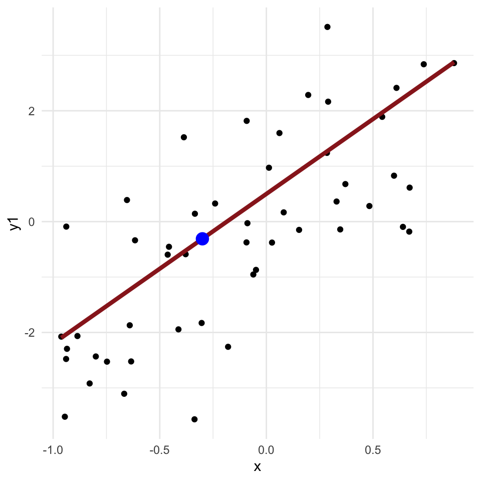
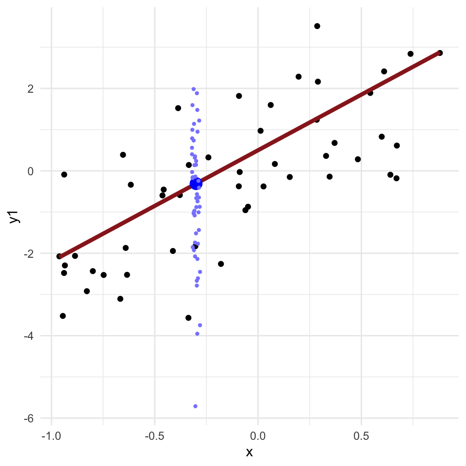
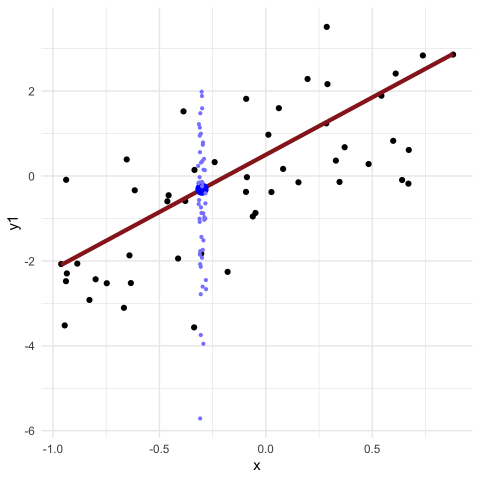
- We want to know how \(y\) changes (on average) with \(x\), and how much variance there is in \(y\)

dnorm
igraph and
ggnetworklibrary("igraph")
library("ggnetwork")
# Here we define the edges
# -+ is an arrow you want to draw (+ is the arrowhead)
# Nodes are created implicitly; name it here and it will be added
gr = graph_from_literal(a-+"E(y)", b-+"E(y)", s-+y, x-+"E(y)", "E(y)"-+y)
# Here we define two attributes, type and source
# These are assigned to nodes using the V (for Vertex) function
# The order is defined by the order the nodes appear when the graph is created
V(gr)$type = c("stochastic", "deterministic", "stochastic",
"stochastic", "stochastic", "deterministic")
V(gr)$source = c("unknown", "unknown", "unknown",
"unknown", "known", "known")
# Here we define an optional layout, telling ggnetwork where to put each node
# The matrix should have one row per node, and columns are x and y coordinates
# If you skip this, ggnetwork will try to make a pretty graph by itself
layout = matrix(c(0.5,2, 0.5,1, 1,2, 1.5,2, 1.25,0, 0,2),
byrow=TRUE, ncol=2)
n = ggnetwork(gr, layout=layout)
(pl = ggplot(n, aes(x = x, y = y, xend = xend, yend = yend)) +
geom_edges(colour="gray50", arrow=arrow(length = unit(6, "pt"),
type = "closed")) +
theme_blank() + geom_nodes(aes(color=type, shape = source), size=6) +
geom_nodelabel(aes(label = name), fontface = "bold", nudge_x=-0.1))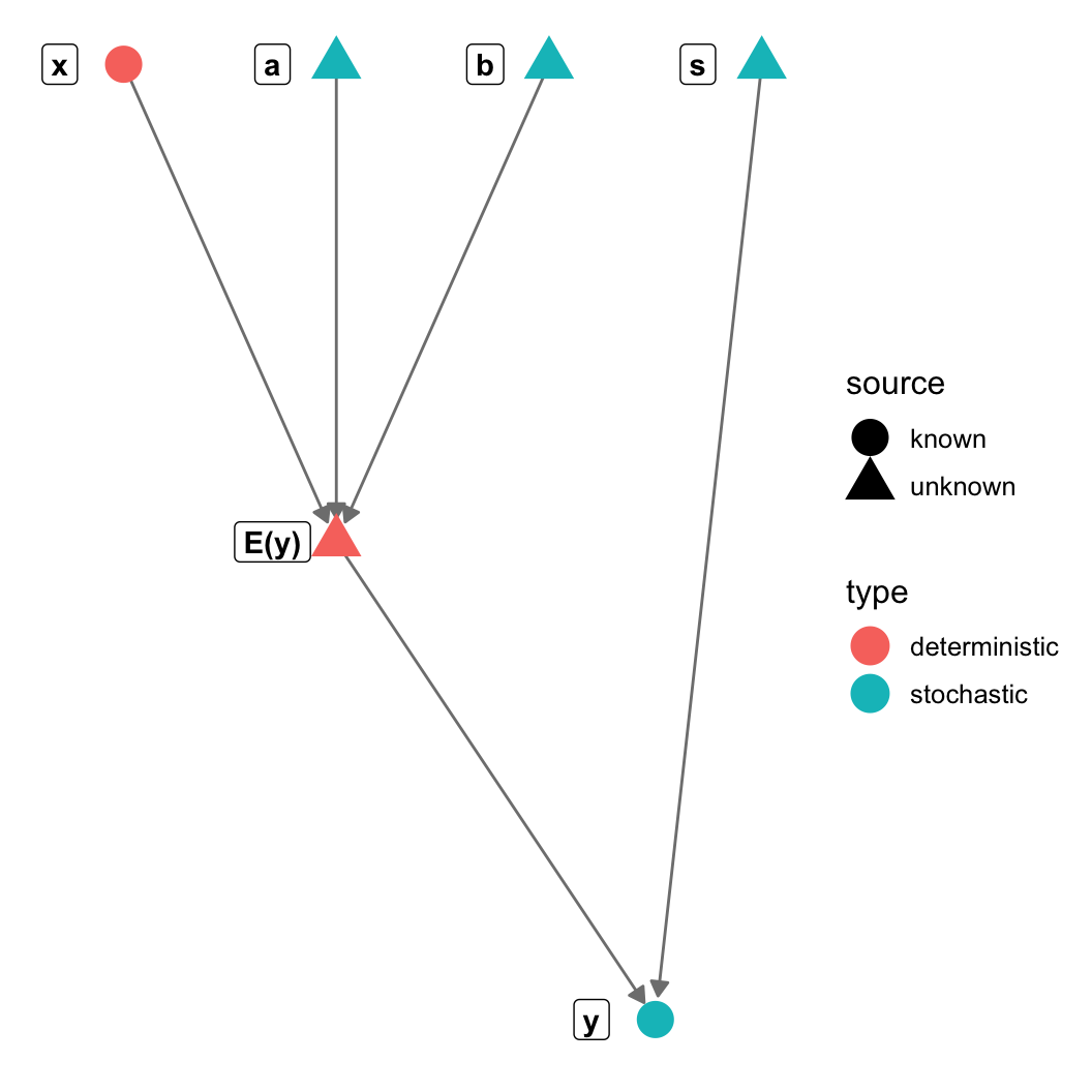
~ symbol (stochastic
nodes)= symbol (deterministic
unknowns)data block (everything else)data and on the left side of
~
y. I will define the distribution of
y (place it on the left side of ~).
y has two dependencies (eta
and s); these should appear on the right side of the
expression for y.declare the variable (i.e., tell Stan
what kind of variable y is: a vector with
length n)

These are guidelines not strict rules…

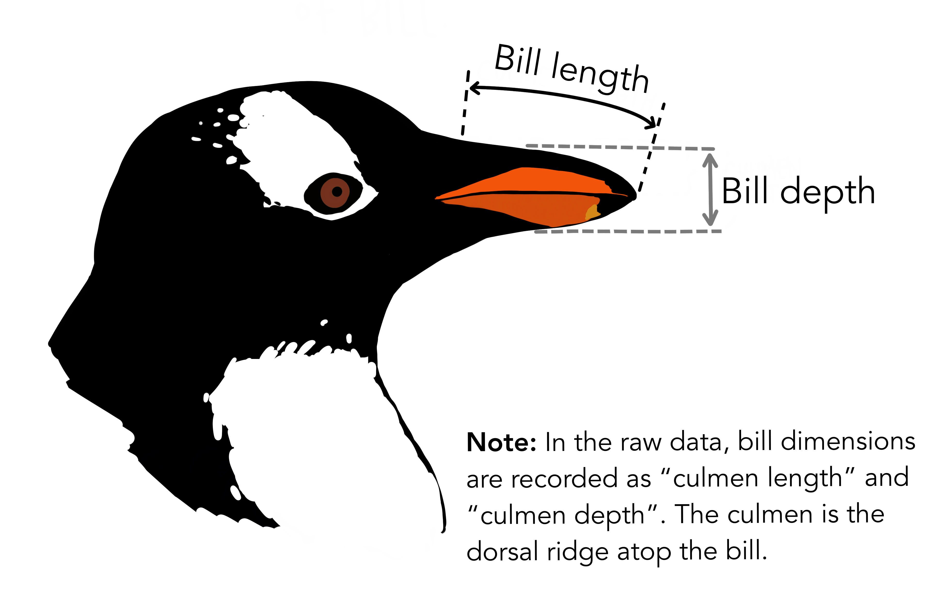
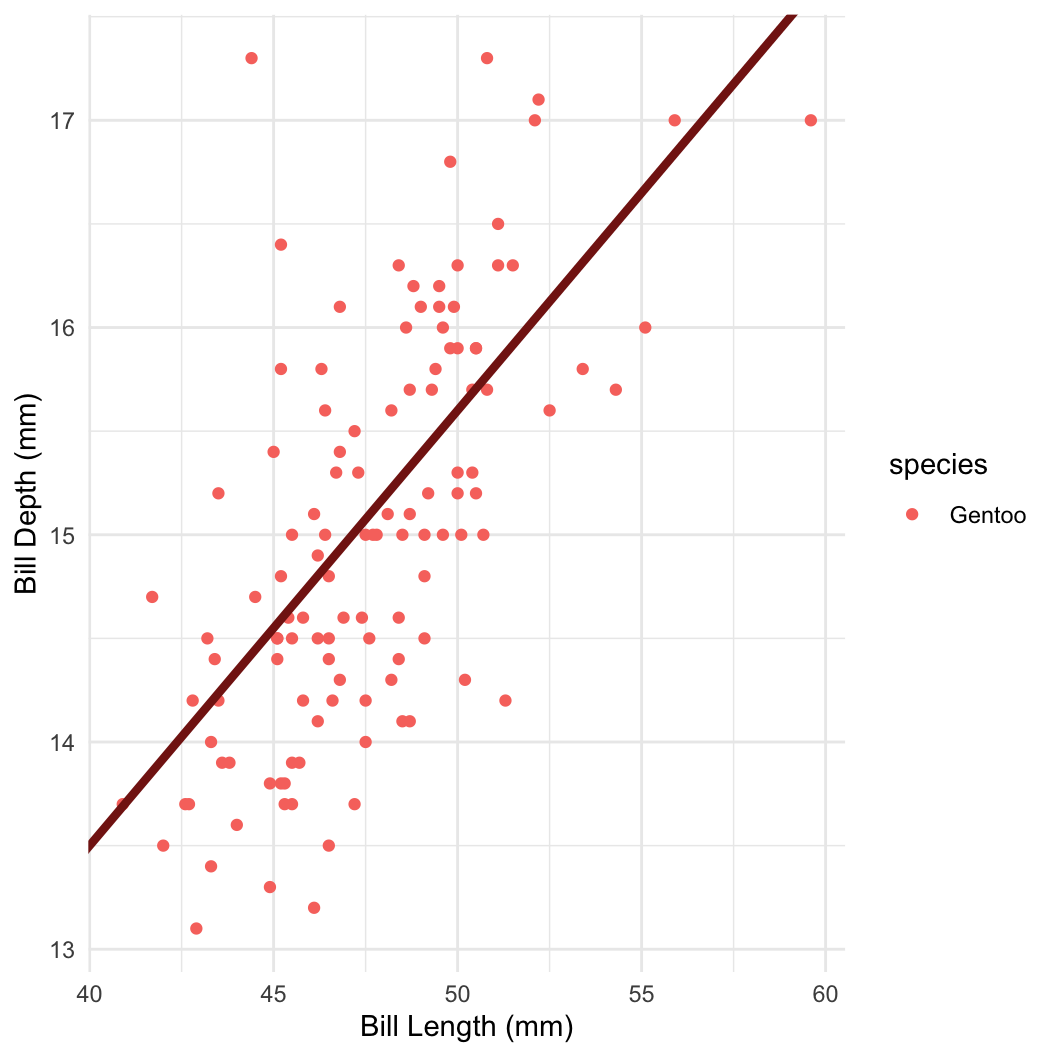
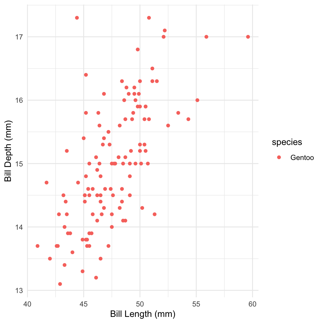
penguins = as.data.frame(palmerpenguins::penguins)
penguins = subset(penguins, complete.cases(penguins) & species == "Gentoo")
peng_dat = with(penguins, list(
bill_len = bill_length_mm,
bill_depth = bill_depth_mm,
n = length(bill_length_mm)
))
peng_fit = sampling(peng_lm, data = peng_dat, refresh = 0)
print(peng_fit, pars = c("a", "b", "s"))
## Inference for Stan model: anon_model.
## 4 chains, each with iter=2000; warmup=1000; thin=1;
## post-warmup draws per chain=1000, total post-warmup draws=4000.
##
## mean se_mean sd 2.5% 25% 50% 75% 97.5% n_eff Rhat
## a 5.00 0.03 1.08 2.88 4.24 5.02 5.76 7.02 993 1
## b 0.21 0.00 0.02 0.17 0.19 0.21 0.23 0.26 989 1
## s 0.76 0.00 0.05 0.66 0.72 0.75 0.79 0.86 1555 1
##
## Samples were drawn using NUTS(diag_e) at Sun Jan 25 18:14:14 2026.
## For each parameter, n_eff is a crude measure of effective sample size,
## and Rhat is the potential scale reduction factor on split chains (at
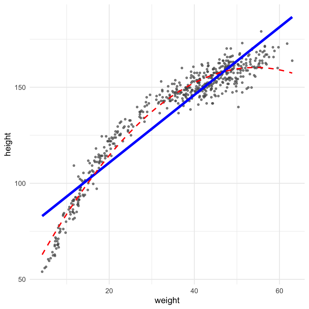
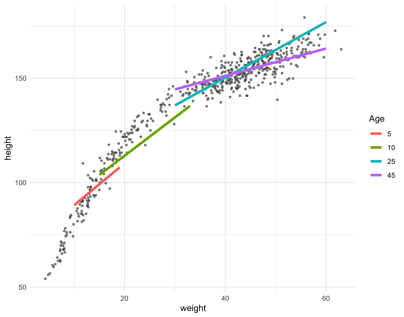
## convergence, Rhat=1).\[ \mathbb{E}(y) = a + b_1x + b_2x^2 \]
Dataset: Nancy Howell (Univ. Toronto) | Measurements of the Dobe !Kung people | Republished in McElreath 2020


library(data.table)
kung = fread("https://github.com/rmcelreath/rethinking/raw/master/data/Howell1.csv")
(pl = ggplot(data = kung, aes(x = weight, y = height)) + geom_point(col = "#555555aa", size = 0.9) +
    geom_smooth(method = "lm", col = "blue", linewidth = 1.5, se = FALSE) +
    geom_smooth(method = "lm", col = "red", linewidth = 0.8, lty = 2, formula = y~x+I(x^2), se = FALSE) +
    theme_minimal())
\[ \mathbb{E}(y) = a + b_1x + b_2x^2 \]
Important: Always remember main effects if including interactions
\[ \mathbb{E}(height) = a + b_1 \times weight + b_2 \times age + b_3 \times weight \times age \]
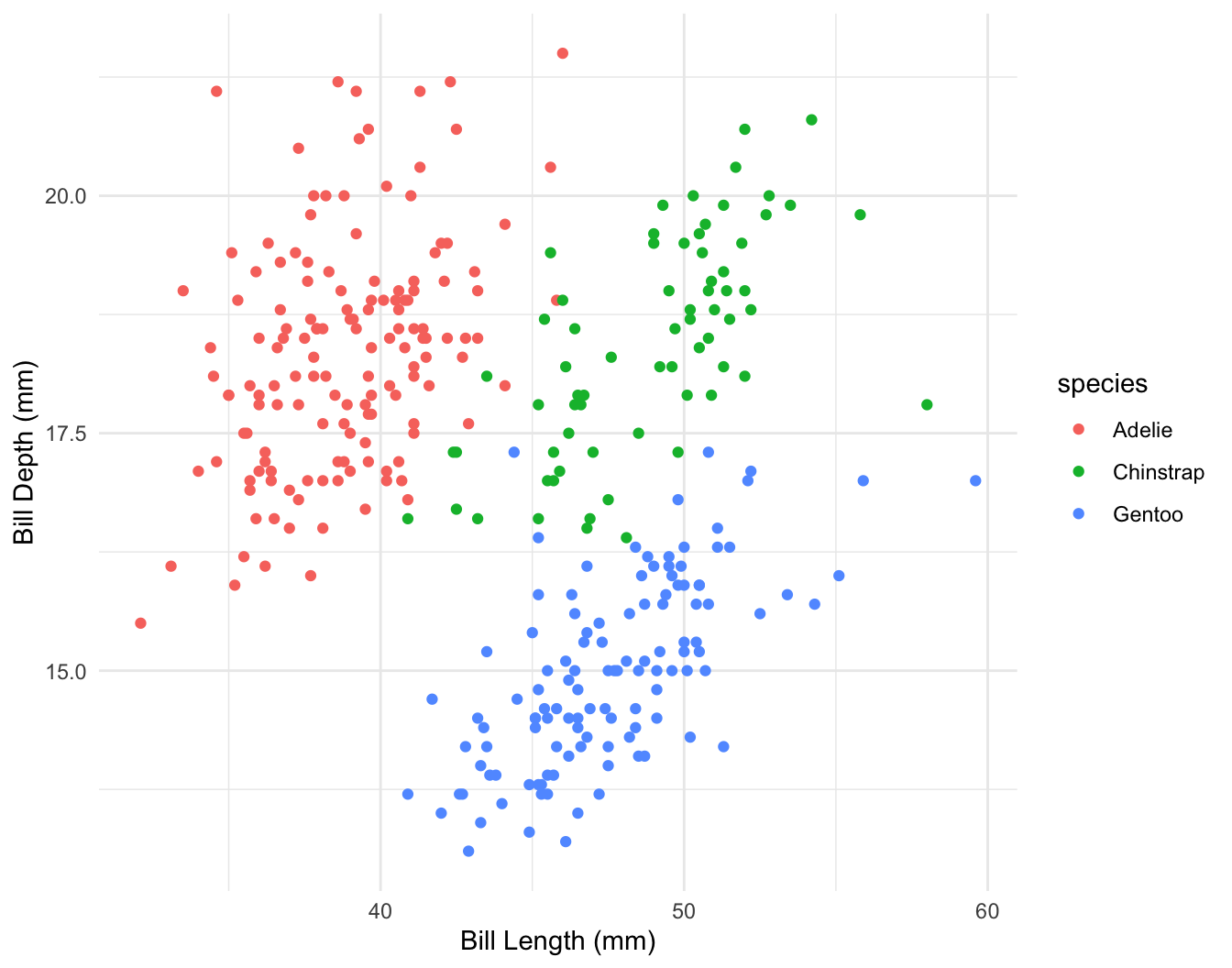
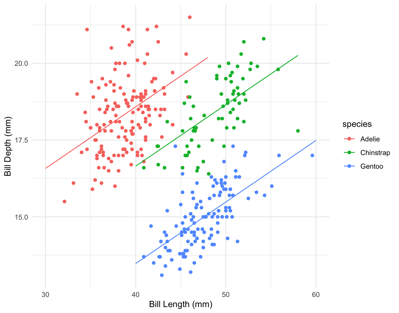
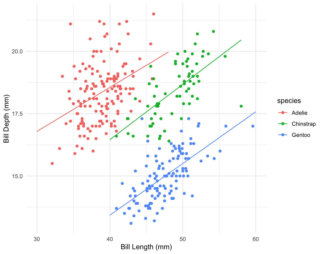
\[ depth = a + b_1 \times length + b_2 \times species?? \]
\[ depth = a + b_1 \times length + b_2 \times chinstrap + b_3 \times gentoo + b_4 \times chinstrap \times length + b_5 \times gentoo \times length \]
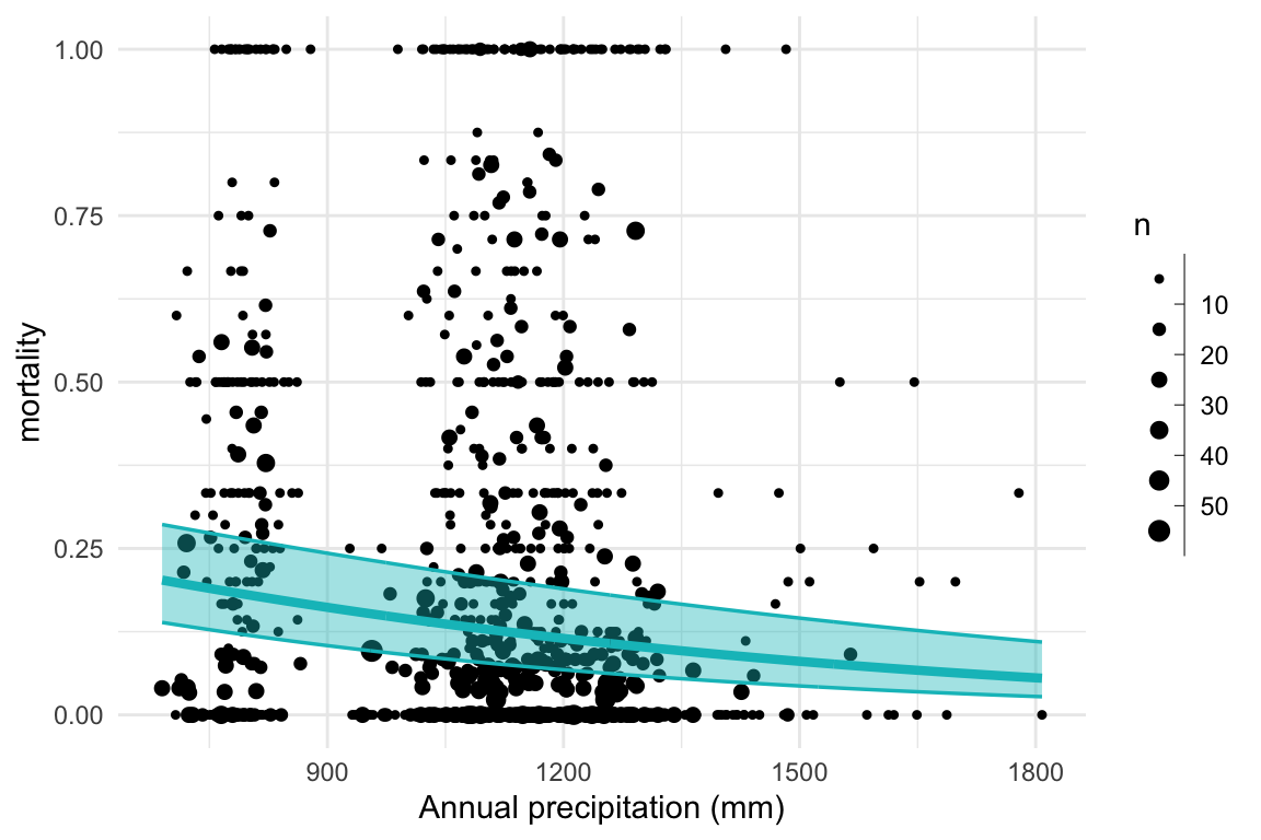
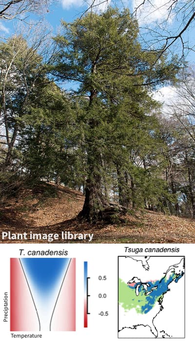
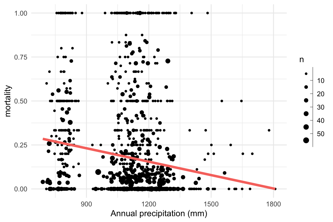
Research question: Does mortality decrease with increasing precipitation?
Dataset: Talluto et al 2017
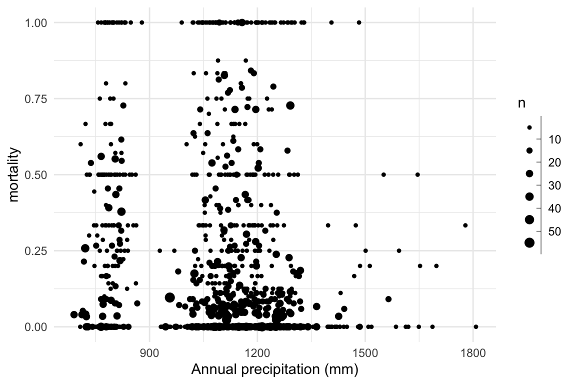
Research question: Does mortality decrease with increasing precipitation?
We can visualise this by computing the proportion of trees that died in each plot.
Dataset: Talluto et al 2017

Research question: Does mortality decrease with increasing precipitation?
Research question: Does mortality decrease with increasing precipitation?

Research question: Does mortality decrease with increasing precipitation?
\[ \begin{aligned} \eta_i & = \mathbb{E}(d_i|n_i) = a + b \times precip_i \\ d_i & \sim \mathrm{Binomial}(n_i, \eta_i) \end{aligned} \]
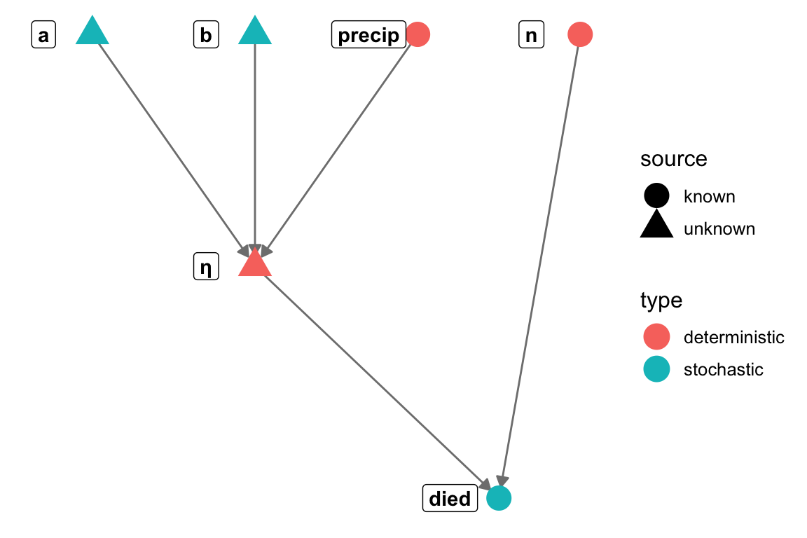
Research question: Does mortality decrease with increasing precipitation? \[ \begin{aligned} \eta_i & = \mathbb{E}(d_i|n_i) = a + b \times precip_i \\ d_i & \sim \mathrm{Binomial}(n_i, \eta_i) \end{aligned} \]
# drop NAs from the dataset, drop plots with no trees
tsuga_stan_dat = with(tsuga[n > 0 & complete.cases(tsuga), ], list(
    died = died,
    n = n,
    precip = tot_annual_pp
))
tsuga_stan_dat$nobs = length(tsuga_stan_dat$n)
tsuga_fit1 = sampling(mort_binom1, data = tsuga_stan_dat, refresh = 0)
## Error in eval(expr, envir) : Initialization failed.
## character(0)
## error occurred during calling the sampler; sampling not done

tsuga_fit1 = sampling(mort_binom1, data = tsuga_stan_dat, refresh = 0,
                      init = list(list(a = 0.46, b = -2.5e-4)), chains=1)
## Warning: There were 871 divergent transitions after warmup. See
## https://mc-stan.org/misc/warnings.html#divergent-transitions-after-warmup
## to find out why this is a problem and how to eliminate them.
## Warning: Examine the pairs() plot to diagnose sampling problems
## Warning: The largest R-hat is 1.77, indicating chains have not mixed.
## Running the chains for more iterations may help. See
## https://mc-stan.org/misc/warnings.html#r-hat
## Warning: Bulk Effective Samples Size (ESS) is too low, indicating posterior means and medians may be unreliable.
## Running the chains for more iterations may help. See
## https://mc-stan.org/misc/warnings.html#bulk-ess
## Warning: Tail Effective Samples Size (ESS) is too low, indicating posterior variances and tail quantiles may be unreliable.
## Running the chains for more iterations may help. See
## https://mc-stan.org/misc/warnings.html#tail-ess
Research question: Does mortality decrease with increasing precipitation?
Problem: This system cannot be linear!
\[ \begin{aligned} \eta_i & = \mathbb{E}(d_i|n_i) = a + b \times precip_i \\ d_i & \sim \mathrm{Binomial}(n_i, \eta_i) \end{aligned} \]

Research question: Does mortality decrease with increasing precipitation?
Problem: This system cannot be linear!
Solution: Transform the linear equation to fit the response using a link function
\[ \begin{aligned} \eta & = a + b \times precip \\ \mathcal{f}(p) & = \mathcal{f}(\mathbb{E}[d|n]) = \eta & \mathrm{or} \\ p & = \mathbb{E}[d|n] = \mathcal{f}^{-1}(\eta) \\ d & \sim \mathrm{Binomial}(n, p) \end{aligned} \]
Research question: Does mortality decrease with increasing precipitation?
Problem: This system cannot be linear!
Solution: Transform the linear equation to fit the response using a link function
Here we need a sigmoid function. A common one for binomial problems is the log odds, or logit function.
\[ \begin{aligned} \ln \frac{p}{1-p} & = \eta = a + b \times precip \\ p & = \frac{e^{\eta}}{1 + e^{\eta}} & \\ d & \sim \mathrm{Binomial}(n, p) \end{aligned} \]

Research question: Does mortality decrease with increasing precipitation? \[ \begin{aligned} \ln \frac{p}{1-p} & = \eta = a + b \times precip \\ p & = \frac{e^{\eta}}{1 + e^{\eta}} & \\ d & \sim \mathrm{Binomial}(n, p) \end{aligned} \]
tsuga_fit2 = sampling(mort_binom2, data = tsuga_stan_dat, refresh = 0)
## Warning: Bulk Effective Samples Size (ESS) is too low, indicating posterior means and medians may be unreliable.
## Running the chains for more iterations may help. See
## https://mc-stan.org/misc/warnings.html#bulk-ess
## Warning: Tail Effective Samples Size (ESS) is too low, indicating posterior variances and tail quantiles may be unreliable.
## Running the chains for more iterations may help. See
## https://mc-stan.org/misc/warnings.html#tail-ess