Bayesian analysis workflow

1. Specify joint posterior graphically, mathematically, and in code

Bayesian analysis workflow

1. Specify joint posterior graphically, mathematically, and in code
2. Draw samples from the joint posterior distribution

Bayesian analysis workflow

1. Specify joint posterior graphically, mathematically, and in code
2. Draw samples from the joint posterior distribution
3. Evaluate/diagnose the model’s performance

Bayesian analysis workflow

1. Specify joint posterior graphically, mathematically, and in code
2. Draw samples from the joint posterior distribution
3. Evaluate/diagnose the model’s performance
4. Perform posterior inference

1. Joint posterior: likelihood

• Choose a generative model (e.g., distribution from which the observations are generated)
  • whenever possible use knowledge of the appropriate processes
  • transform parameters and sample in transformed space to improve behaviour
  • e.g. use log(\(\sigma\)) instead of \(\sigma\) to avoid impossible negative variance in sampler
  • in Stan, this is done by adding variable constraints (real <lower=0> sigma)

1. Joint posterior: likelihood

• Choose a generative model (e.g., distribution from which the observations are generated)
  • whenever possible use knowledge of the appropriate processes
  • transform parameters and sample in transformed space to improve behaviour
  • e.g. use log(\(\sigma\)) instead of \(\sigma\) to avoid impossible negative variance in sampler
  • in Stan, this is done by adding variable constraints (real <lower=0> sigma)
• Models should be specified to be scale independent
  • Easy: scaling your predictors to have mean=0, sd=1
  • Hard: scaling outcomes (y); this can change the generative model!
  • Prefer to transform outcomes with the link function

1. Joint posterior: priors

• Any unknowns must have a prior
  • (or possibly a hierarchical generative model and hyperpriors)
• Prefer regularising priors to vague priors
  • Normal(0, 5) instead of Normal(0,500)
• Avoid improper priors: Uniform(-Inf, Inf)
  • This is the default in Stan if you forget to specify it!

1. Joint posterior: priors

• Avoid hard boundaries
  • No: Uniform(0, 1000)
  • Yes: Exponential(0.1)
• With informative priors, specify reasonable initial values
• Begin sampling with weaker priors, gradually strengthen once you know the model is working
• Specify priors for everything—avoid defaults
• Draw out your model as a digraph to make sure you don’t miss anything

GLM in Stan

For this exercise, you will use the birddiv (in vu_advstats_students/data/birddiv.csv) dataset; you can load it directly from github using data.table::fread(). Bird diversity was measured in 1-km^2 plots in multiple countries of Europe, investigating the effects of habitat fragmentation and productivity on diversity. We will consider a subset of the data. Specificially, we will ask how various covariates are associated with the diversity of birds specializing on different habitat types. The data have the following potential predictors:

• Grow.degd: growing degree days, a proxy for how warm the climate is.
• For.cover: Forest cover near the sampling location
• NDVI: normalized difference vegetation index, a proxy for productivity
• For.diver: Forest diversity in the forested area nearby
• Agr.diver: Diversity of agricultural landscapes
• For.fragm: Index of forest fragmentation

All of the above variables are standardized to a 0-100 scale. Consider this when choosing priors.

Your response variable will be richness, the bird species richness in the plot. Additionally, you have an indicator variable hab_type. This is not telling you what habitat type was sampled (plots included multiple habitats). Rather, this is telling you what type of bird species were counted for the richness measurement: so hab_type == "forest" & richness == 7 indicates that 7 forest specialists were observed in that plot.

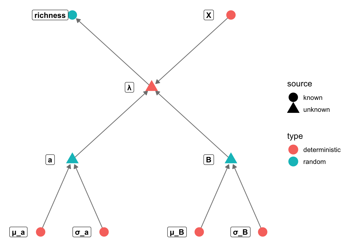
Build one or more generalised linear models for bird richness. Your task should be to describe two things: (1) how does richness vary with climate, productivity, fragmentation, or habitat diversity, and (2) do these relationships vary depending on what habitat bird species specialize on.

1. Specify joint posterior

1. Specify joint posterior

1. Specify joint posterior

data {
    int <lower=0> n; // number of data points
    int <lower=0> k; // number of x-variables
    int <lower=0> richness [n];
    matrix [n,k] X;
    
    // prior hyperparams
    real mu_a;
    real mu_b;
    real <lower=0> sigma_a;
    real <lower=0> sigma_b;
}
parameters {
    real a;
    vector [k] B;
}
transformed parameters {
    vector <lower=0> [n] lambda;
    lambda = exp(a + X * B);
}
model {
    richness ~ poisson(lambda);
    a ~ normal(mu_a, sigma_a);
    B ~ normal(mu_b, sigma_b);
}
generated quantities {
    int r_predict [n];
    for(i in 1:n)
        r_predict[i] = poisson_rng(lambda[i]);
    r_predict = poisson_rng(lambda);
}

2. Sample from joint posterior

• Start with a small run (10s-100s of iterations) to catch errors, make sure nothing surprising happens
• Increase to a few thousand to view convergence
• Select starting values and run until convergence (1.000s for Stan, 10.000s—100.000s or more for Metropolis)
• Use multiple chains (it will be needed for step 3)

2. Sample from the joint posterior

First we compile the model and prepare the data.

library(rstan)
bird_div_glm = stan_model("stan/bird_div_glm.stan")

library(data.table)
birds = fread("../vu_advstats_students/data/birddiv.csv")

# stan can't handle NAs
birds = birds[complete.cases(birds)]

# turn predictors into a matrix
X = as.matrix(birds[, c("Grow.degd", "For.cover", "NDVI", 
                        "For.diver", "Agr.diver", "For.fragm")])

# Remove the scale from X, make the model scale independent
X_scaled = scale(X)

2. Sample from the joint posterior

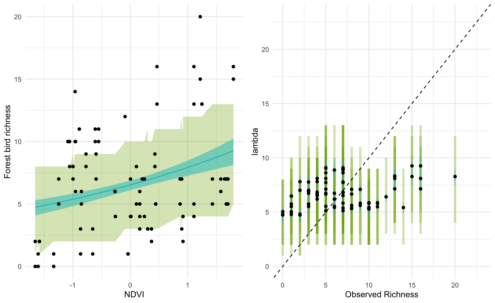
Next we fit an initial model using only NVDI as a predictor.

which_forest = which(birds$hab_type == "forest")
standat1 = list(
    n = length(which_forest), 
    k = 1,
    richness = birds$richness[which_forest],
    X = X_scaled[which_forest, "NDVI", drop=FALSE],
    mu_a = 0,
    mu_b = 0,
    # these prior scales are still SUPER vague
    # exp(20) is a possible intercept under this prior!
    sigma_a = 10,
    sigma_b = 5
)

fit1 = sampling(bird_glm, data = standat1, iter=5000, 
   chains = 4, refresh = 0)

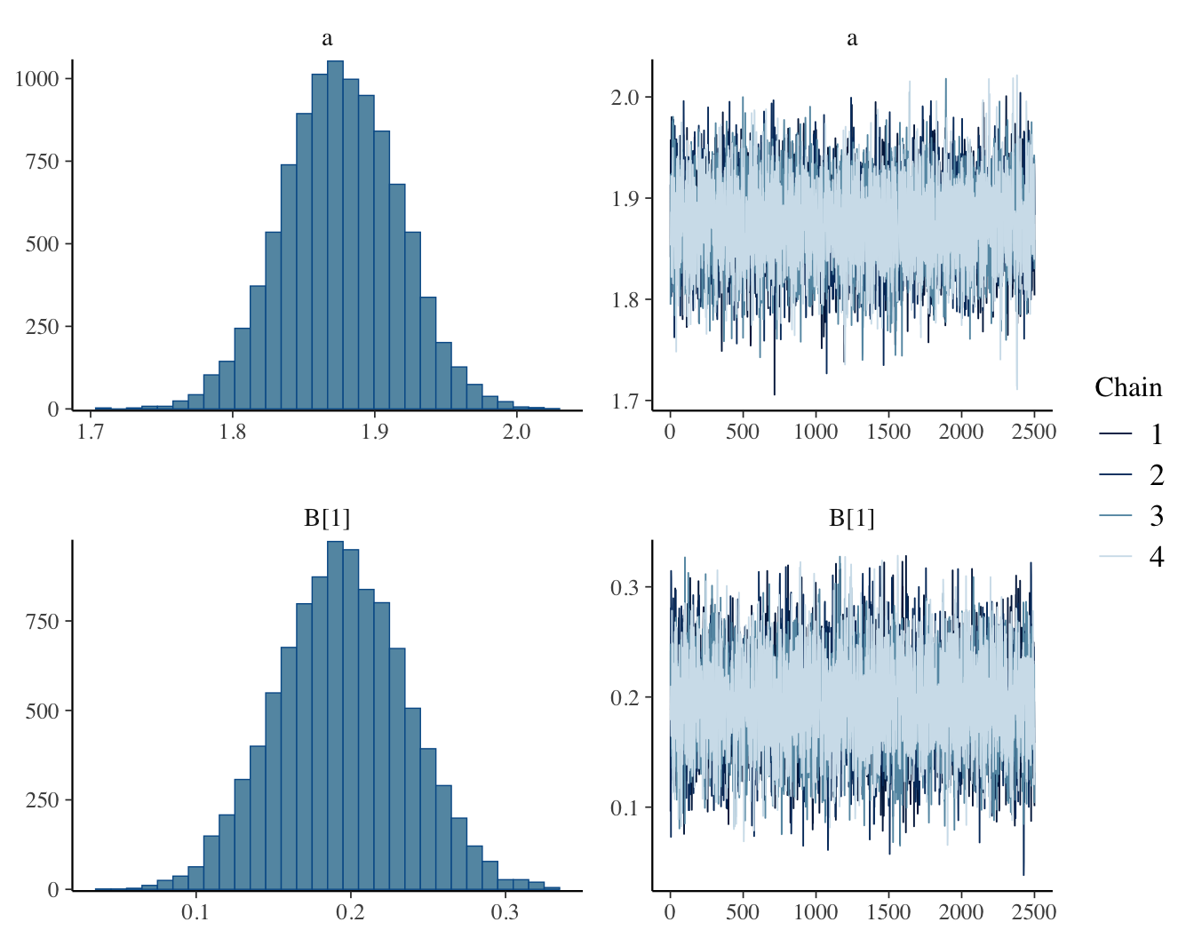
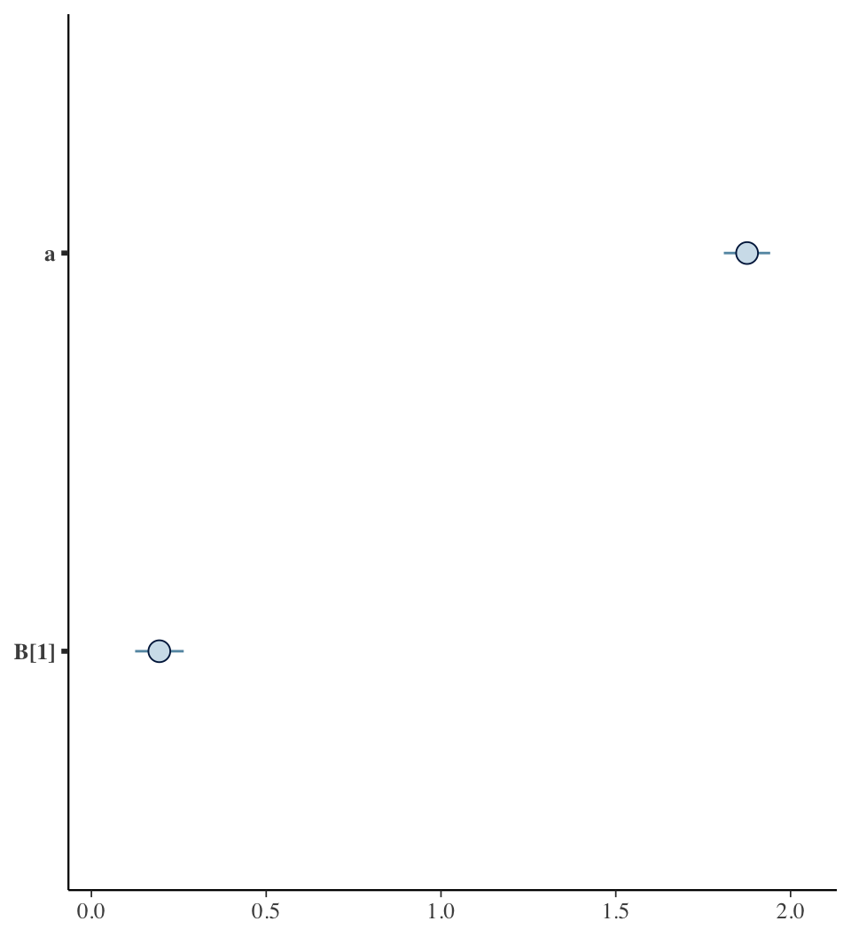
2. Sample from the joint posterior

## Inference for Stan model: anon_model.
## 4 chains, each with iter=5000; warmup=2500; thin=1; 
## post-warmup draws per chain=2500, total post-warmup draws=10000.
## 
##      mean se_mean   sd 2.5%  25%  50%  75% 97.5% n_eff Rhat
## a    1.88       0 0.04 1.80 1.85 1.88 1.90  1.96  7254    1
## B[1] 0.19       0 0.04 0.11 0.17 0.19 0.22  0.28  7365    1
## 
## Samples were drawn using NUTS(diag_e) at Mon Dec  2 13:01:18 2024.
## For each parameter, n_eff is a crude measure of effective sample size,
## and Rhat is the potential scale reduction factor on split chains (at 
## convergence, Rhat=1).

2. Sample from the joint posterior

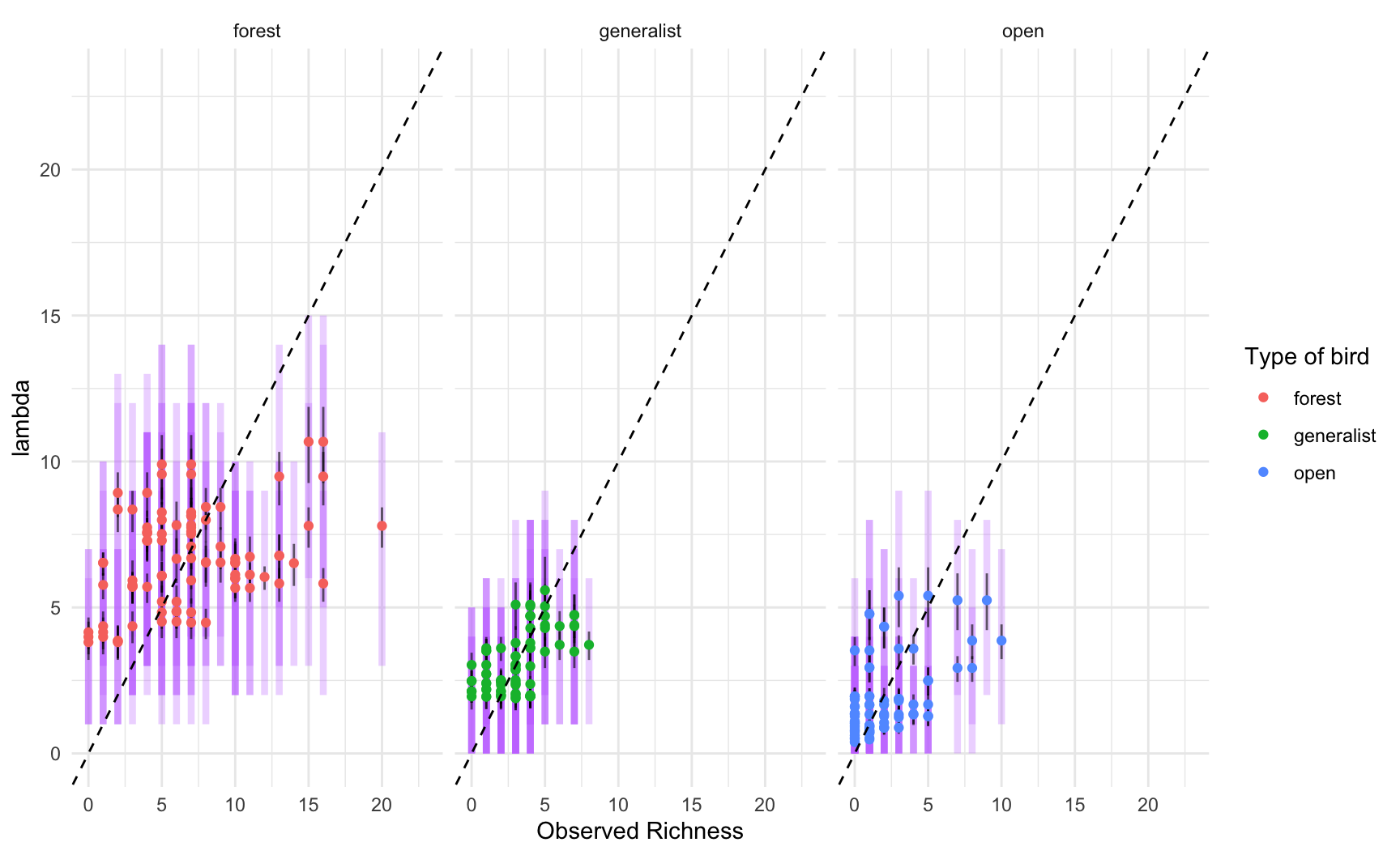
Next, we choose two variables, and try them using birds of different habitat types.

# Second, looking at how two variables influence birds of different types

# grab two variables
X_2 = X_scaled[, c("For.cover", "NDVI")]

# add a categorical variable for bird type
X_2 = cbind(X_2, open=ifelse(birds$hab_type == "open",1, 0))
X_2 = cbind(X_2, generalist=ifelse(birds$hab_type == "generalist",1, 0))

# add interaction terms with the categories
X_2 = cbind(X_2, 
            op_forCov = X_2[,"For.cover"] * X_2[,"open"], 
            op_NDVI = X_2[, "NDVI"] * X_2[,"open"], 
            ge_forCov = X_2[,"For.cover"] * X_2[,"generalist"],
            ge_NDVI = X_2[,"NDVI"] * X_2[,"generalist"])

head(X_2)
##       For.cover       NDVI open generalist op_forCov op_NDVI ge_forCov ge_NDVI
## [1,]  1.1895779  0.4284131    0          0         0       0         0       0
## [2,] -1.3937570 -0.8660731    0          0         0       0         0       0
## [3,] -0.4034797 -1.2463741    0          0         0       0         0       0
## [4,] -1.0985427 -0.9977157    0          0         0       0         0       0
## [5,] -1.3937570 -1.5827942    0          0         0       0         0       0
## [6,]  1.1930054  0.2090086    0          0         0       0         0       0

2. Sample from the joint posterior

Next, we choose two variables, and try them using birds of different habitat types.

standat2 = list(
    n = length(birds$richness), 
    k = ncol(X_2),
    richness = birds$richness,
    X = X_2, 
    mu_a = 0,
    mu_b = 0,
    # these prior scales are still SUPER vague (exp(20) is a possible intercept under this prior!)
    sigma_a = 10,
    sigma_b = 5
)

fit2 = sampling(bird_glm, data = standat2, iter=5000, 
   chains = 4, refresh = 0)

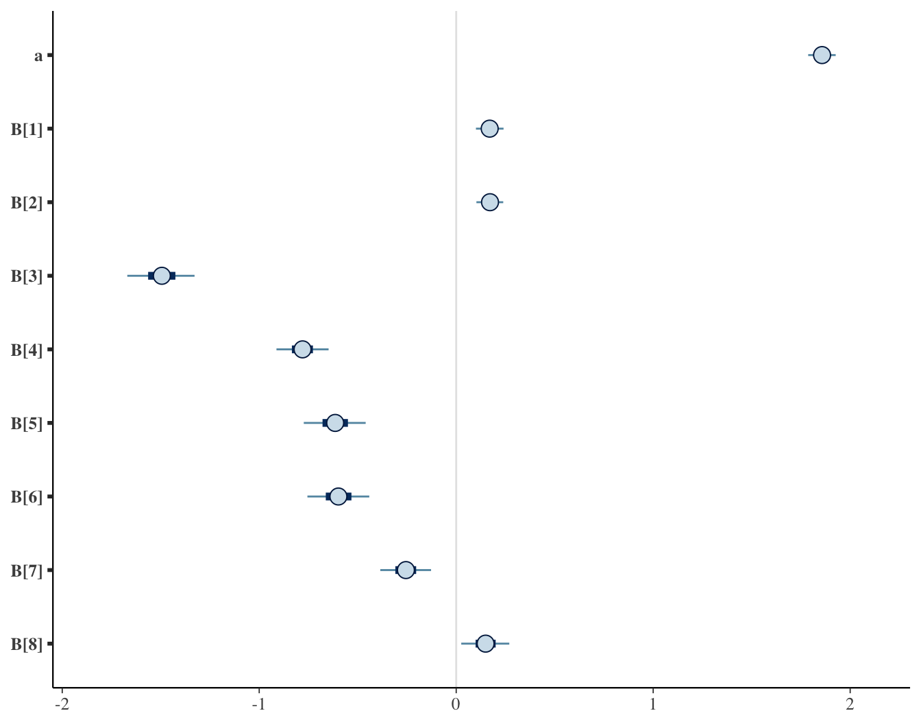
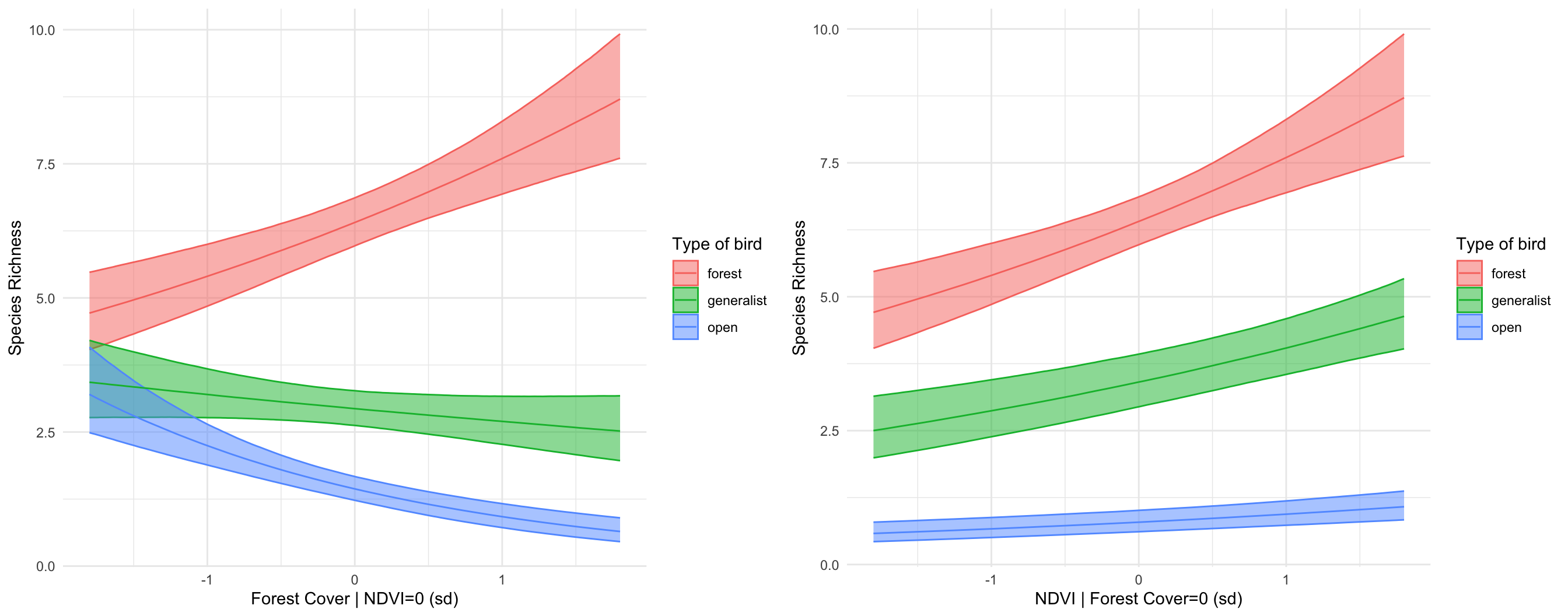
2. Sample from the joint posterior

## Inference for Stan model: anon_model.
## 4 chains, each with iter=5000; warmup=2500; thin=1; 
## post-warmup draws per chain=2500, total post-warmup draws=10000.
## 
##       mean se_mean   sd  2.5%   25%   50%   75% 97.5% n_eff Rhat
## a     1.86       0 0.04  1.77  1.83  1.86  1.88  1.94  8121    1
## B[1]  0.17       0 0.04  0.09  0.14  0.17  0.20  0.25  7279    1
## B[2]  0.17       0 0.04  0.09  0.14  0.17  0.20  0.25  7975    1
## B[3] -1.50       0 0.10 -1.70 -1.56 -1.49 -1.43 -1.30  8538    1
## B[4] -0.78       0 0.08 -0.94 -0.83 -0.78 -0.73 -0.62  8346    1
## B[5] -0.61       0 0.10 -0.80 -0.68 -0.61 -0.55 -0.43  8142    1
## B[6] -0.60       0 0.10 -0.79 -0.66 -0.60 -0.53 -0.41  8717    1
## B[7] -0.26       0 0.08 -0.41 -0.31 -0.26 -0.20 -0.10  8060    1
## B[8]  0.15       0 0.07  0.00  0.10  0.15  0.20  0.29  8507    1
## 
## Samples were drawn using NUTS(diag_e) at Mon Dec  2 13:01:24 2024.
## For each parameter, n_eff is a crude measure of effective sample size,
## and Rhat is the potential scale reduction factor on split chains (at 
## convergence, Rhat=1).

3. Evaluate the model fit

library(bayesplot)
## Use as.array if you want to keep different mcmc chains separate
## This is ideal for diagnostics
## For inference, you usually want to lump all chains
## In this case, you use as.matrix
samp1_pars = as.array(fit1, pars=c('a', 'B'))
mcmc_combo(samp1_pars, c("hist", "trace"))

3. Evaluate the model fit

print(fit1, pars = c('a', 'B'))
## Inference for Stan model: anon_model.
## 4 chains, each with iter=5000; warmup=2500; thin=1; 
## post-warmup draws per chain=2500, total post-warmup draws=10000.
## 
##      mean se_mean   sd 2.5%  25%  50%  75% 97.5% n_eff Rhat
## a    1.88       0 0.04 1.80 1.85 1.88 1.90  1.96  7254    1
## B[1] 0.19       0 0.04 0.11 0.17 0.19 0.22  0.28  7365    1
## 
## Samples were drawn using NUTS(diag_e) at Mon Dec  2 13:01:18 2024.
## For each parameter, n_eff is a crude measure of effective sample size,
## and Rhat is the potential scale reduction factor on split chains (at 
## convergence, Rhat=1).

4. Inference: parameter estimates

mcmc_intervals(samp1_pars)

samp2_pars = as.array(fit2, pars=c('a', 'B'))
mcmc_intervals(samp2_pars)

4. Inference: Retrodiction

# extract the samples
samp1_lam = as.matrix(fit1, pars='lambda')

# compute the posterior distribution of the residual deviance
dev1 = apply(samp1_lam, 1, function(x) -2 * sum(dpois(standat1$richness, x, log = TRUE)))

# compute posterior distribution of dispersion parameter, which is just 
# deviance/(n - k)
# here k is 2, we have an intercept and one slope
# if phi > 1, we have overdispersion and need a better model
phi = dev1 / (length(standat1$richness) - 2)
quantile(phi, c(0.05, 0.95))
##       5%      95% 
## 6.144344 6.210879

4. Inference: Improve the model

# extract the samples
samp2_lam = as.matrix(fit1, pars='lambda')

# compute the posterior distribution of the residual deviance
dev2 = apply(samp2_lam, 1, function(x) -2 * sum(dpois(standat2$richness, x, log = TRUE)))

phi = dev2 / (length(standat2$richness) - 9)
quantile(phi, c(0.05, 0.95))
##       5%      95% 
## 7.367951 8.149738

4. Inference: Partial Response Curves

• How does richness respond to the individual variables, holding other variables constant?

4. Inference: Response Surfaces