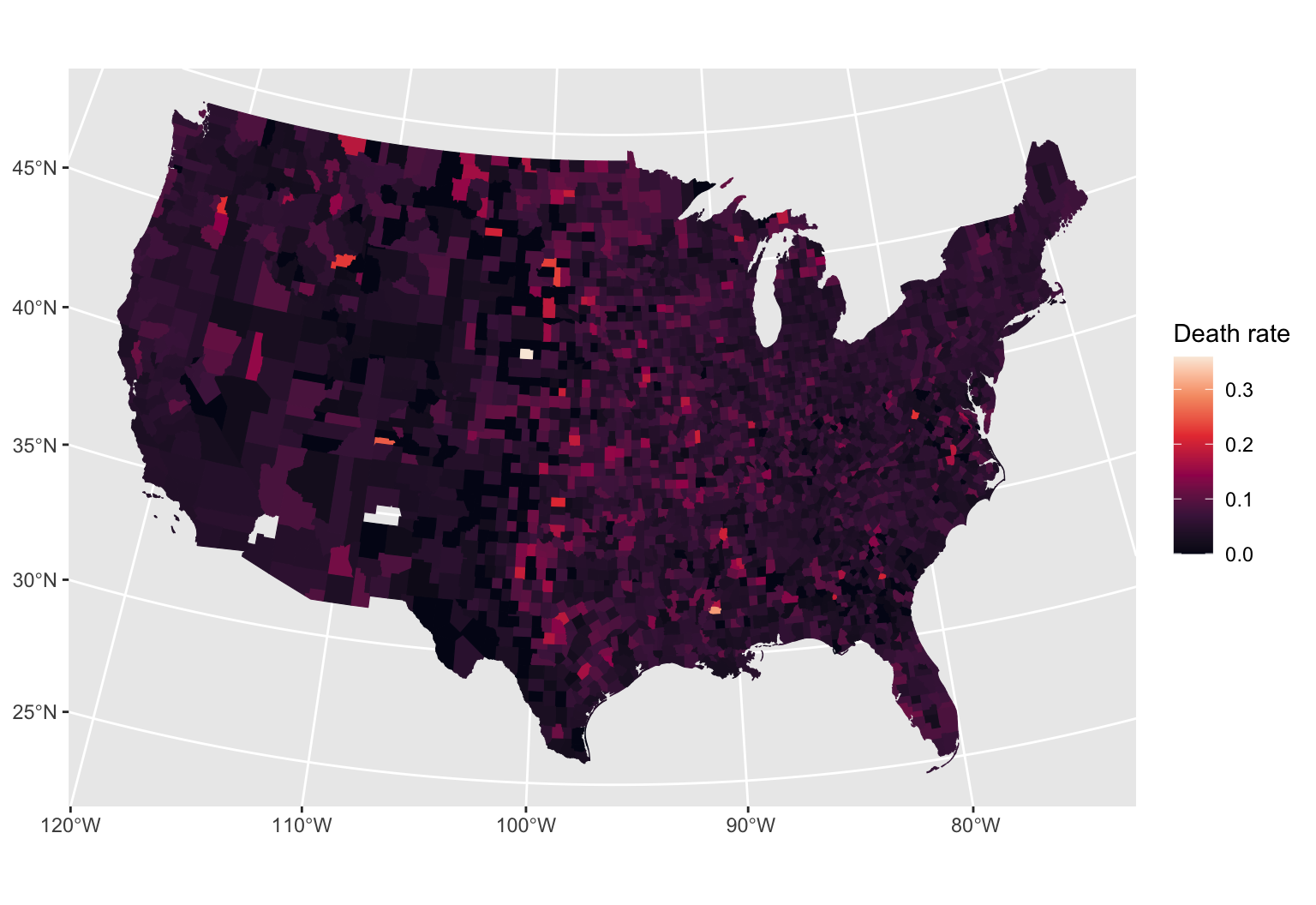
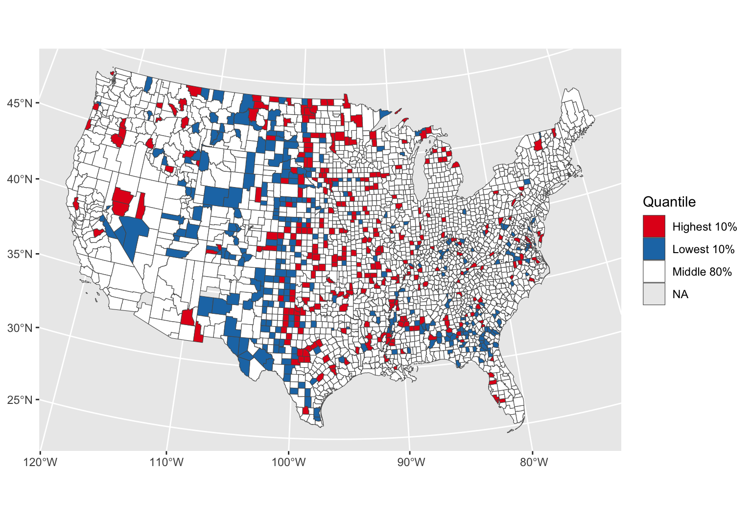
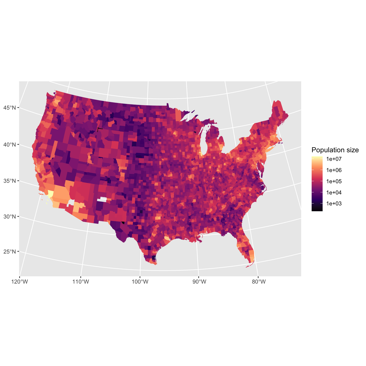
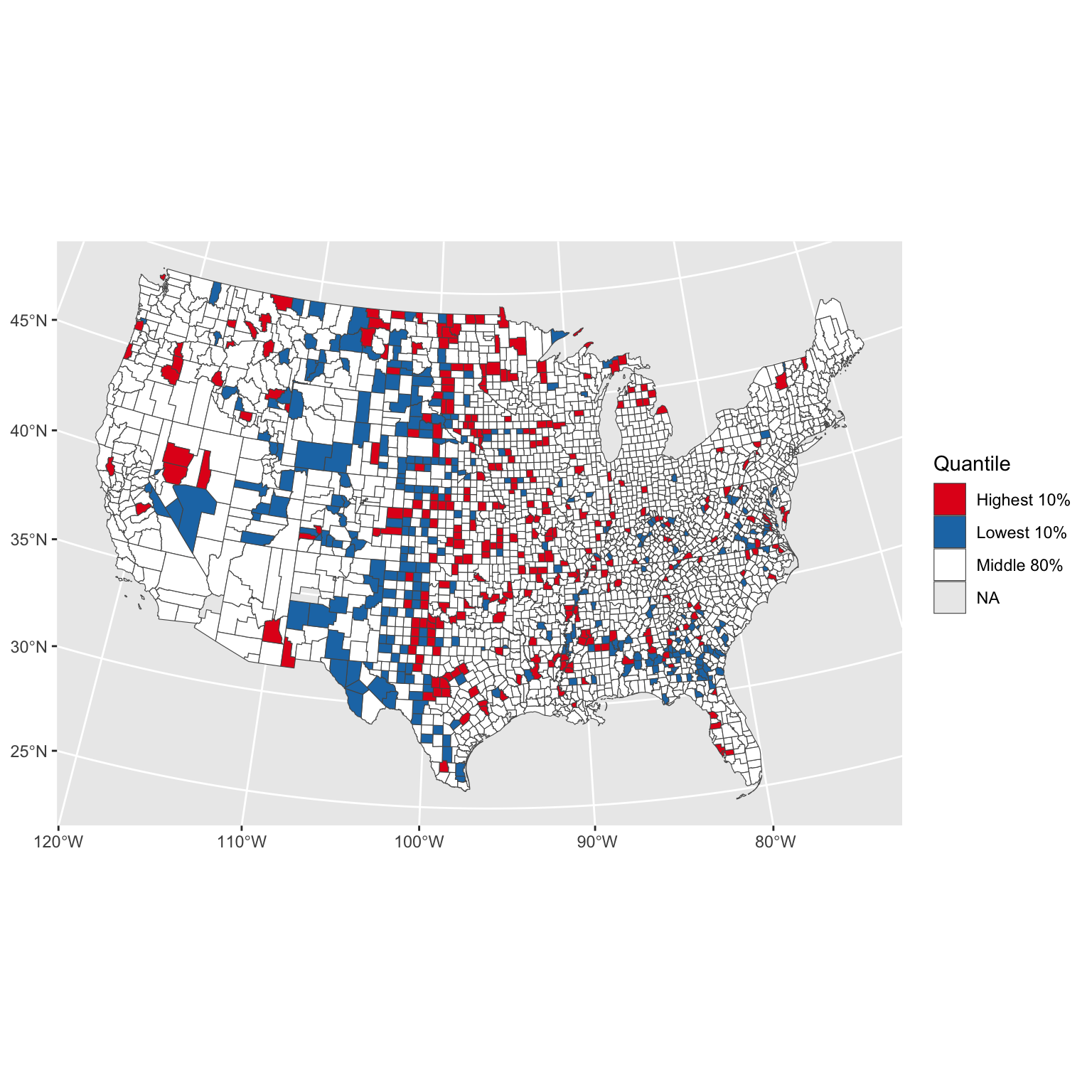
Kidney cancer death rates in the US

Counties in the extreme quantiles are also among the smallest!
How can we estimate county-specific rates in a reasonable way?

`Mean population size by quantile

Highest 10%	32328
Lowest 10%	22125
Middle 80%	208246

# Overall rate for the whole country
(mean_rate = with(counties, 
                  sum(kc_deaths, na.rm = TRUE) / sum(population, na.rm = TRUE)))
## [1] 4.983687e-05


# expected value when population size = 25000
mean_rate * 25000
## [1] 1.245922

Kidney cancer Stan model: global/constant rate

Our data are counts, suggesting Poisson
- We don’t use binomial in part because we care about death rate, not probability
Here we build a model accounting for exposure (population size)
We assume mortality rate \(\lambda\) is constant for the entire dataset
- \(\lambda\) is pooled across units (county)

library(data.table)
(cancer = readRDS("../vu_advstats_students/data/us_k_cancer.rds"))
##         state     county kidney_cancer_deaths population death_rate_per_1000
##        <char>     <char>                <int>      <int>               <num>
##    1: alabama    autauga                    2      61921          0.03229922
##    2: alabama    baldwin                    7     170945          0.04094884
##    3: alabama    barbour                    0      33316          0.00000000
##    4: alabama       bibb                    0      30152          0.00000000
##    5: alabama     blount                    3      88342          0.03395893
##   ---                                                                       
## 6256: wyoming sweetwater                    2     104192          0.01919533
## 6257: wyoming      teton                    0      26751          0.00000000
## 6258: wyoming      uinta                    1      52910          0.01890002
## 6259: wyoming   washakie                    2      22814          0.08766547
## 6260: wyoming     weston                    0      17802          0.00000000

Kidney cancer Stan model: global/constant rate

Our data are counts, suggesting Poisson
- We don’t use binomial in part because we care about death rate, not probability
Here we build a model accounting for exposure (population size)
We assume mortality rate \(\lambda\) is constant for the entire dataset
- \(\lambda\) is pooled across units (county)

data {
    int <lower = 1> n;
    int <lower = 0> deaths [n];
    int <lower = 0> population [n];
    real <lower = 0> alpha;
    real <lower = 0> beta;
}
transformed data {
    // cancer is rare, lets make the numbers more reasonable
    vector <lower = 0> [n] exposure;
    for(i in 1:n)
        exposure[i] = population[i] / 1000.0;
}
parameters {
    real <lower = 0> lambda;
}
model {
    deaths ~ poisson(exposure * lambda);
    lambda ~ gamma(alpha, beta);
}

Kidney cancer Stan model: global/constant rate

Our data are counts, suggesting Poisson
- We don’t use binomial in part because we care about death rate, not probability
Here we build a model accounting for exposure (population size)
We assume mortality rate \(\lambda\) is constant for the entire dataset
- \(\lambda\) is pooled across units (county)
- Interpretation of \(\lambda\): cancer deaths per five years per 1000 people

Question: Is there geographic variation in cancer rates?

library(rstan)
cancer_pooled = stan_model("stan/kidney_cancer_pooled.stan")

cancer = cancer[complete.cases(cancer)]
cancer_data_stan = list(
    n = nrow(cancer),
    deaths = cancer$kidney_cancer_deaths,
    population = cancer$population,
    alpha = 0.01, # extremely vague priors, probably too vague!
    beta = 0.01
)
cancer_p_fit = sampling(cancer_pooled, data = cancer_data_stan, refresh = 0)
quantile(as.matrix(cancer_p_fit, pars = "lambda")[,1], c(0.05, 0.95))
##         5%        95% 
## 0.04989637 0.05063215

Kidney cancer Stan model: rates per county

We assume mortality rate \(\lambda\) is independent for each county
- \(\lambda\) is unpooled across units (county)
This model has a lot of parameters, and doesn’t fit well
Max of 2 observations per lambda!

data {
    int <lower = 1> n;
    int <lower = 1> n_counties;
    int <lower = 0> deaths [n];
    int <lower = 0> population [n];
    int <lower = 0, upper = n_counties> county_id [n];
    real <lower = 0> alpha;
    real <lower = 0> beta;
}
transformed data {
    // cancer is rare, lets make the numbers more reasonable
    vector <lower = 0> [n] exposure;
    for(i in 1:n)
        exposure[i] = population[i] / 1000.0;
}
parameters {
    vector <lower = 0> [n_counties] lambda;
}
model {
    for(i in 1:n) {
        int j = county_id[i];
        deaths[i] ~ poisson(exposure[i] * lambda[j]);
    }
    lambda ~ gamma(alpha, beta);
}

Kidney cancer Stan model: partial pooling

We can use the overall rate for the whole country as a prior for individual counties
Areas with few observations will use the whole country as a slight reality check
\(\lambda\) is partially pooled

data {
    int <lower = 1> n;
    int <lower = 1> n_counties;
    int <lower = 0> deaths [n];
    int <lower = 0> population [n];
    int <lower = 0, upper = n_counties> county_id [n];

    // hyper-hyper parameters, for the hyperprior
    real <lower = 0> a_alpha;
    real <lower = 0> a_beta;
    real <lower = 0> b_alpha;
    real <lower = 0> b_beta;
}
transformed data {
    // cancer is rare, lets make the numbers more reasonable
    vector <lower = 0> [n] exposure;
    for(i in 1:n)
        exposure[i] = population[i] / 1000.0;
}
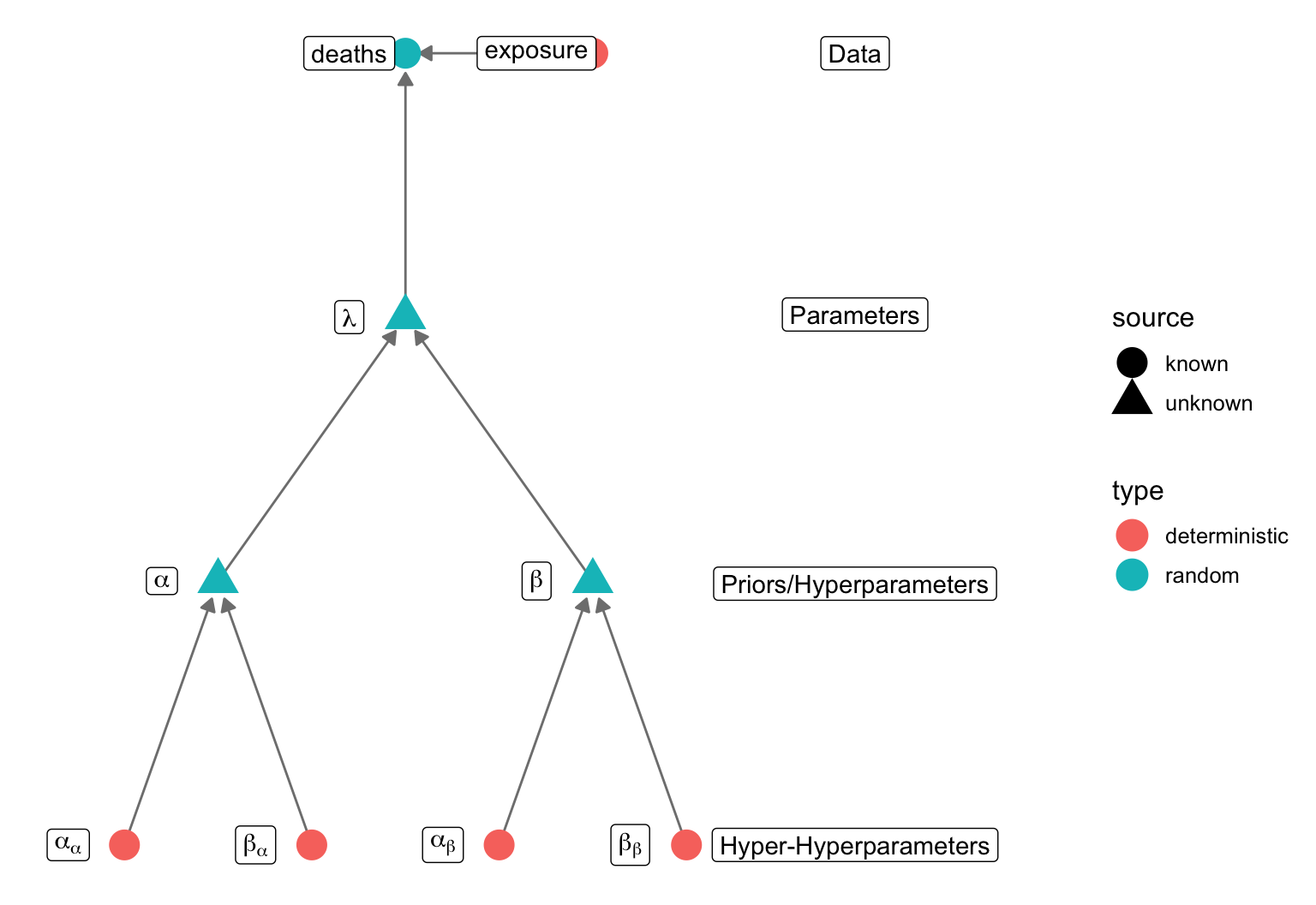
parameters {
    vector <lower = 0> [n_counties] lambda;
    
    // prior hyperparameters for lambda are now parameters we will estimate!
    real <lower = 0> alpha;
    real <lower = 0> beta;
    
}
model {
    for(i in 1:n) {
        int j = county_id[i];
        deaths[i] ~ poisson(exposure[i] * lambda[j]);
    }
    
    // prior for lambda
    lambda ~ gamma(alpha, beta);
    
    // hyperpriors for alpha and beta
    alpha ~ gamma(a_alpha, a_beta);
    beta ~ gamma(b_alpha, b_beta);
}
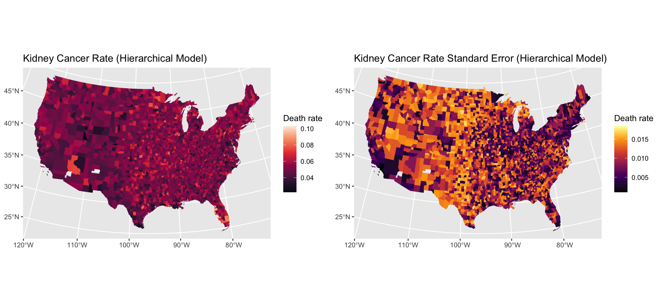
generated quantities {
    // save the overal mean and variance in cancer rate
    real lambda_mu = alpha/beta;
    real lambda_var = alpha/beta^2;
}

Kidney cancer Stan model: partial pooling

We can use the overall rate for the whole country as a prior for individual counties
Areas with few observations will use the whole country as a slight reality check
\(\lambda\) is partially pooled
Parameters with limited information can borrow strength from the rest of the dataset
We must take care when choosing the hyperprior parameters
- this cancer is rare, less than one per 1000 on average
- we choose a range for alpha and beta that is wide, but makes mostly impossible values very unlikely

mean(cancer$death_rate_per_1000/(cancer$population/1000))
## [1] 0.00214512

sd(cancer$death_rate_per_1000/(cancer$population/1000))
## [1] 0.009377513

alpha_a = 0.01
beta_a = 1

# our hyperparameter alpha has a 99% prob of being between these two values
(a_int = qgamma(c(0.01, 0.99), alpha_a, beta_a))
## [1] 5.660738e-201  2.650526e-01


alpha_b = 0.8
beta_b = 0.4
# our hyperparameter beta has a 99% prob of being between these two values
(b_int = (round(qgamma(c(0.01, 0.99), alpha_b, beta_b), 2)))
## [1]  0.01 10.32


## what would the mean lambda look like at these extremes?
round(matrix(c(a_int[1] / b_int[1], a_int[2]/b_int[1], a_int[1] / b_int[2], a_int[2] / b_int[2]), nrow = 2, 
       dimnames = list(c("min a", "max a"), c("min b", "max b"))),2)
##       min b max b
## min a  0.00  0.00
## max a 26.51  0.03


cancer_data_stan$a_alpha = alpha_a
cancer_data_stan$b_alpha = alpha_b
cancer_data_stan$a_beta = beta_a
cancer_data_stan$b_beta = beta_b

Kidney cancer Stan model: partially pooled rates per county

We can use the overall rate for the whole country as a prior for individual counties
Areas with few observations will use the whole country as a slight reality check
\(\lambda\) is partially pooled
Parameters with limited information can borrow strength from the rest of the dataset
We must take care when choosing the hyperprior parameters
- this cancer is rare, less than one per 1000 on average
- we choose a range for alpha and beta that is wide, but makes mostly impossible values very unlikely

library(rstan)
cancer_unpooled = stan_model("stan/kidney_cancer_ppooled.stan")

cancer$county_id = as.integer(factor(cancer$county))
cancer_data_stan$county_id = cancer$county_id
cancer_data_stan$n_counties = max(cancer$county_id)

cancer_ppool_fit = sampling(cancer_ppooled, data = cancer_data_stan, refresh = 0, iter = 5000)
cancer_ppool_samps = as.matrix(cancer_ppool_fit, pars = "lambda")
quants = t(apply(cancer_ppool_samps , 2, quantile, c(0.05, 0.95)))
head(quants)
##            
## parameters          5%        95%
##   lambda[1] 0.04955227 0.10113314
##   lambda[2] 0.05096910 0.09156240
##   lambda[3] 0.04524905 0.09524071
##   lambda[4] 0.03334261 0.05388143
##   lambda[5] 0.03801103 0.07283501
##   lambda[6] 0.03671909 0.04921456


# quantile interval for the overall mean
round(rbind(pooled = quantile(as.matrix(cancer_p_fit, pars = "lambda"), c(0.05, 0.95)),
    partial_pooled = quantile(as.matrix(cancer_ppool_fit, pars = "lambda_mu"), c(0.05, 0.95))), 4)
##                    5%    95%
## pooled         0.0499 0.0506
## partial_pooled 0.0508 0.0527

Kidney cancer Stan model: partially pooled maps

Precipitation-mortality relationships in Tsuga

We return to the mortality of trees in North American forests
The dataset contains information for multiple species and years
- there is replication within units
For now, we focus on Tsuga canadensis

trees = fread("../vu_advstats_students/data/treedata.csv")
tsuga = trees[grep("Tsuga", species_name)]
# remove NAs
tsuga = tsuga[complete.cases(tsuga), ]
head(tsuga)
##        n  died  year     species_name annual_mean_temp tot_annual_pp   prior_mu
##    <int> <int> <int>           <char>            <num>         <num>      <num>
## 1:     5     3  1989 Tsuga canadensis         3.849333     1003.0000 0.02222166
## 2:     6     0  1989 Tsuga canadensis         3.452000     1076.1333 0.02222166
## 3:     3     0  1997 Tsuga canadensis         3.620000     1099.4000 0.03245619
## 4:     4     4  1989 Tsuga canadensis         4.596000      989.4667 0.02222166
## 5:     3     0  1994 Tsuga canadensis         4.244667     1116.2000 0.02816339
## 6:     7     0  2002 Tsuga canadensis         4.730000     1137.2667 0.04108793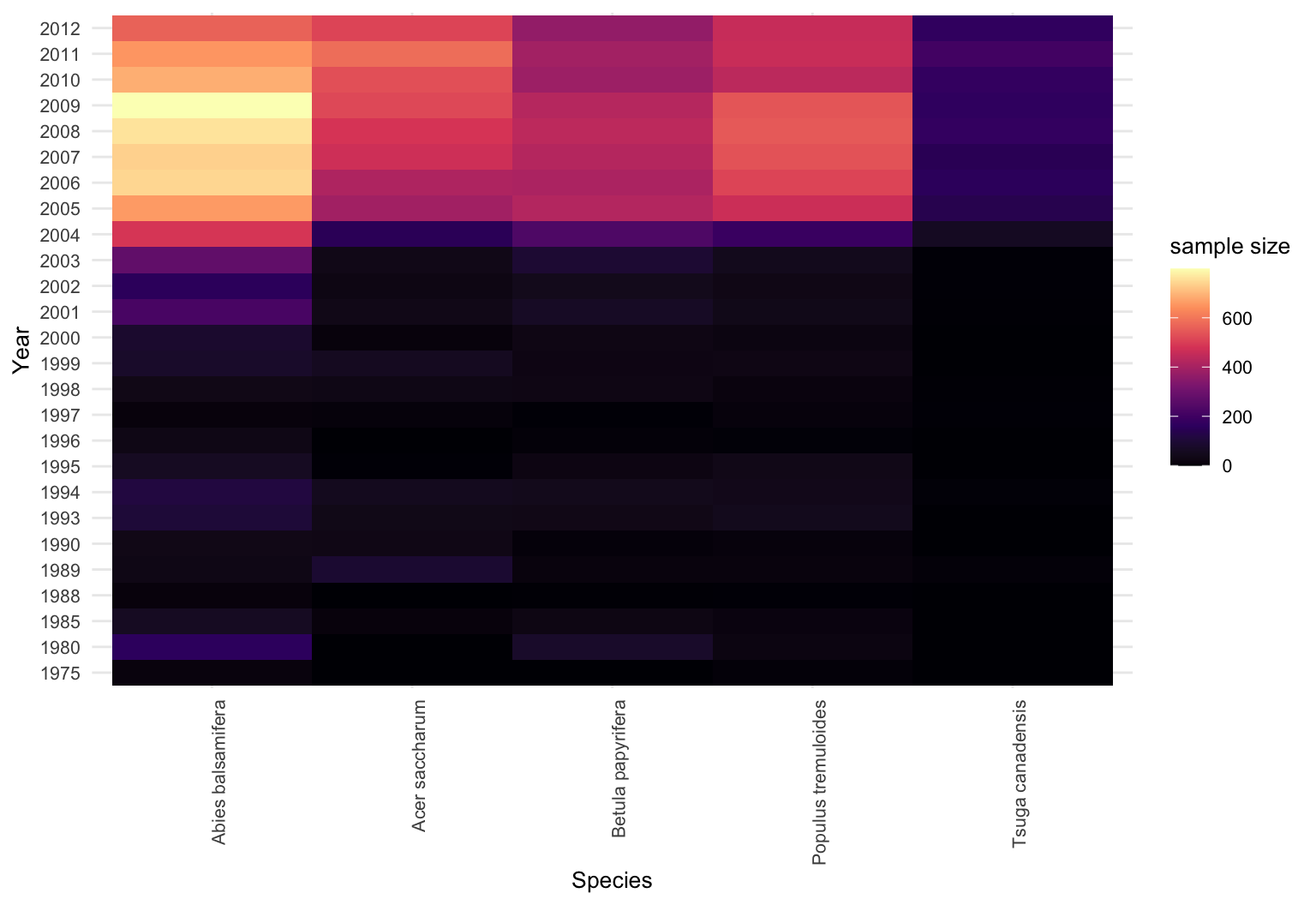

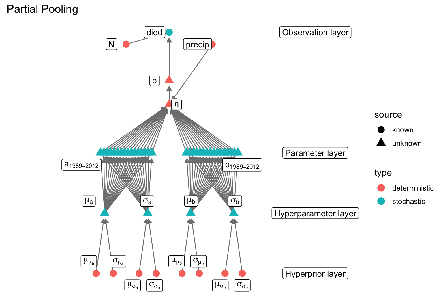
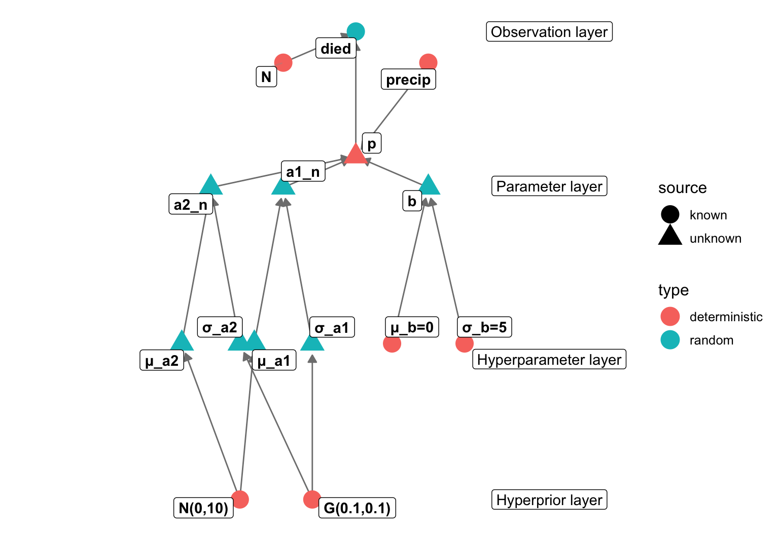
Precipitation-mortality relationships in Tsuga: H1

Question: Does mortality of Tsuga canadensis vary with precipitation?
- The species generally prefers moist conditions
Hypothesis 1: The precipitation-mortality relationship is the same across all years (Complete pooling, 2 params)

Precipitation-mortality relationships in Tsuga: H2

Question: Does mortality of Tsuga canadensis vary with precipitation?
- The species generally prefers moist conditions
Hypothesis 1: The precipitation-mortality relationship is the same across all years (Complete pooling, 2 params)
Hypothesis 2: The average survival varies by year, but the slope between precipitation and mortality is constant (Unpooled intercepts, pooled slopes, 17 params)
- Sample size by year ranges from 1 to 208

Precipitation-mortality relationships in Tsuga: H3

Question: Does mortality of Tsuga canadensis vary with precipitation?
- The species generally prefers moist conditions
Hypothesis 1: The precipitation-mortality relationship is the same across all years (Complete pooling, 2 params)
Hypothesis 2: The average survival varies by year, but the slope between precipitation and mortality is constant (Unpooled intercepts, pooled slopes, 17 params)
- Sample size by year ranges from 1 to 208
Hypothesis 3: There is a different regression line for each year (No pooling, 32 parameters)

Pooled model: code

data {
    // number of data points
    int <lower=0> n; 
    
    // number of trees in each plot
    int <lower=1> n_trees [n]; 

    // number died
    int <lower=0> died [n]; 
    vector [n] precip;
}
parameters {
    real a;
    real b;
}
transformed parameters {
    vector <lower=0, upper=1> [n] p;
    p = inv_logit(a + b * precip);
}
model {
    died ~ binomial(n_trees, p);
    a ~ normal(0, 10);
    b ~ normal(0, 5);
}
generated quantities {
    // we use generated quantities to keep track of log likelihood and
    // deviance, useful for model selection
    // and also to perform poserior predictive simulations
    real deviance = 0;
    vector [n] loglik;
    int ppd_died [n];
    for (i in 1:n) {
        loglik[i] = binomial_lpmf(died[i] | n_trees[i], p[i]);
        deviance += loglik[i];
        ppd_died[i] = binomial_rng(20, p[i]);
    }
    deviance = -2 * deviance;
}

Pooled models trade accuracy for precision

All data for a single set of estimates
- highly precise parameter estimates

Pooled models trade accuracy for precision

All data for a single set of estimates
- highly precise parameter estimates
High prediction errors for individual groups
Groups with small samples biased towards the mean

Unpooled model: code

data {
    // not the complete program, only differences from pooled model

    // grouping variables
    // year_id is an integer starting at 1 (the earliest year)
    // ending at n_groups (the latest year)
    // we use this value as an index for any group-level effects
    int <lower=1> n_groups;
    int <lower=1, upper = n_groups> year_id [n];
}
parameters {
    // one intercept per group
    vector [n_groups] a;
}
transformed parameters {
    // a is different for each data point, depending on the group
    // so we need a loop to compute this
    for(i in 1:n) {
        int gid = year_id[i];
        p[i] = inv_logit(a[gid] + b * precip[i]);
    }
}

Unpooled model: code

# factor variables must be converted to integers for stan
standat$year_id = as.integer(standat$year)

# we also need to tell stan how many groups (i.e., years) there are
standat$n_groups = max(standat$year_id)

fit_unpooled = sampling(tsuga_unpooled, chains=4, iter=3000, refresh=0, 
                        data = standat)

Unpooled models use less data per parameter

Very imprecise, especially for groups with few samples
Prediction to new groups (years) impossible

Compromise: partial pooling

We don’t really expect each year to be independent
- it’s all one species, response to precipitation should be similar
- some years are better or worse than others

Imagine instead there is a population of possible years, each with its own mortality
This population has a true mean and a true variance
The samples we’ve taken will come from that distribution
This can tell us something about all possible years, not just these years

Partial Pooling: Code

data {
    // not the complete program, only differences from pooled model

    // grouping variables
    // year_id is an integer starting at 1 (the earliest year)
    // ending at n_groups (the latest year)
    // we use this value as an index for any group-level effects
    int <lower=1> n_groups;
    int <lower=1, upper = n_groups> year_id [n];
}
parameters {
    // one intercept and one slope per group
    vector [n_groups] a;
    vector [n_groups] b;

    // hyperparameters describe higher-level structure in the data
    // in this case both the a's and b's come from populations
    // with their own mean and variance to be estimated from the data
    real a_mu;
    real <lower=0> a_sig;
    real b_mu;
    real <lower=0> b_sig;
}
transformed parameters {
    for(i in 1:n) {
        int gid = year_id[i];
        p[i] = inv_logit(a[gid] + b[gid] * precip[i]);
    }
}
model {
    // The priors are now estimated from the data
    a ~ normal(a_mu, a_sig);
    b ~ normal(b_mu, b_sig);
    
    // hyperpriors describe what we know about higher (group-level) structure
    a_mu ~ normal(0, 20);
    b_mu ~ normal(0, 20);
    // half cauchy is common for hierarchical stdev
    a_sig ~ cauchy(0, 20);
    b_sig ~ cauchy(0, 20);

}

Partial pooling is a compromise

for a given group, we combine the information for this group with information from all groups
balances precision and accuracy
can be best approach for new groups
weak/undersampled groups can “borrow strength” from others

Partial pooling is a compromise

When do we need hierarchical models?

Repeated sampling within units (e.g., samples nested within plots/individuals)
Inference at multiple levels of organisation (e.g., Covariates at multiple spatial scales)
Uneven sampling among units (Number of trees by year)
Accounting for nonindependence of samples

When do we need hierarchical models?

Repeated sampling within units (e.g., samples nested within plots/individuals)
Inference at multiple levels of organisation (e.g., Covariates at multiple spatial scales)
Uneven sampling among units (Number of trees by year)
Accounting for nonindependence of samples
Avoiding pre-averaging
- Don’t: perform repeat samples on a unit, perform analysis on the average
- Do: Build an HM accounting for variability within and among units

When do we need hierarchical models?

Repeated sampling within units (e.g., samples nested within plots/individuals)
Inference at multiple levels of organisation (e.g., Covariates at multiple spatial scales)
Uneven sampling among units (Number of trees by year)
Accounting for nonindependence of samples
Avoiding pre-averaging
- Don’t: perform repeat samples on a unit, perform analysis on the average
- Do: Build an HM accounting for variability within and among units
A common category of HM is often called mixed modeling
- All mixed models are hierarchical, not all hierarchical models are mixed models

Designing hierarchical models in Stan

You must specify data/objects at all levels
Often we use an indexing variable to link observations to their group
This variable must start at 1 and end at n_groups

data {
    // group-level objects
    int <lower=1> n_groups;
    int <lower=1, upper=n_groups> group_id [n];
}
parameters {
    vector [n_groups] a; 
    
    // hyperparameters
    real a_mu;
    real a_sig;
}
transformed parameters {
    pr[i] = inv_logit(a[group_id[i]]);
}
model {
    a ~ normal(a_mu, a_sig);  // hierarchical prior for a
}

Designing hierarchical models in Stan

You must specify data/objects at all levels
Often we use an indexing variable to link observations to their group
This variable must start at 1 and end at n_groups
Multiple non-nested groups are possible

data {
    int n; // number of data points
    int died [n]
    int N[n];
    vector [n] precip;

    // group-level objects
    int <lower=1> n_group1;
    int <lower=1, upper=n_group1> group1_id [n];

    int <lower=1> n_group2;
    int <lower=1, upper=n_group2> group2_id [n];
}
parameters {
    vector [n_group1] a1; 
    vector [n_group2] a2; 
    
    // hyperparameters
    real a1_mu;
    real <lower=0> a1_sig;
    real a2_mu;
    real <lower=0> a2_sig;
}
transformed parameters {
    vector [n] pr;
    for(i in 1:n)
        pr[i] = inv_logit(a1[group1_id[i]] + a2[group2_id[i]] + b*precip[i]);
}
model {
    died ~ binomial(N, pr); // likelihood

    a1 ~ normal(a1_mu, a1_sig);  // hierarchical prior for a1
    a2 ~ normal(a2_mu, a2_sig);  // hierarchical prior for a2

    // hyperpriors
    a1_mu ~ normal(0,10)
    a2_mu ~ normal(0,10)
    a1_sig ~ gamma(0.1, 0.1);
    a2_sig ~ gamma(0.1, 0.1);
}

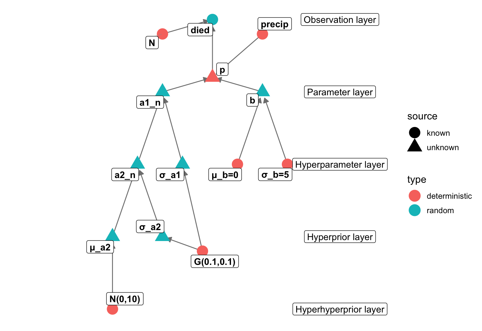
Designing hierarchical models in Stan

Nested groups add an additional hierarchical layer

data {
    int n; // number of data points
    int died [n]
    int N[n];
    vector [n] temperature;

    // group-level objects
    int <lower=1> n_group1;
    int <lower=1, upper=n_group1> group1_id [n];

    int <lower=1> n_group2;
    int <lower=1, upper=n_group2> group2_id [n_group1];
}
parameters {
    vector [n_group1] a1; 
    vector [n_group2] a2; 
    
    // hyperparameters
    real <lower=0> a1_sig;
    real a2_mu;
    real <lower=0> a2_sig;
}
transformed parameters {
    vector [n] pr;
    for(i in 1:n)
        pr[i] = inv_logit(a1[group1_id[i]] + b*precip[i]);
}
model {
    died ~ binomial(N, pr); // likelihood

    for(i in n_group1)
        a1 ~ normal(a2[i], a1_sig);  // hierarchical prior for a1
    // hyperpriors
    a2 ~ normal(a2_mu, a2_sig);  // hierarchical prior for a2
    a1_sig ~ gamma(0.1, 0.1);
    
    // hyperhyperprior
    a2_mu ~ normal(0,10)
}

Posterior predictive distributions

Do we want to predict new observations from a known group?
- e.g: What is the PPD for trees in 1989?
- Use generated quantities block in Stan
Or new observations from an unknown group?
- Simulate new values for each param, drawn from hyper params
- Then simulate the individual observations

sim1 = function(amu, asig, bmu, bsig, N, precip) {
    a = rnorm(length(precip), amu, asig)
    b = rnorm(length(precip), bmu, bsig)
    p = plogis(a + b*precip)
    rbinom(length(precip), N, p)
}

Posterior predictive distributions

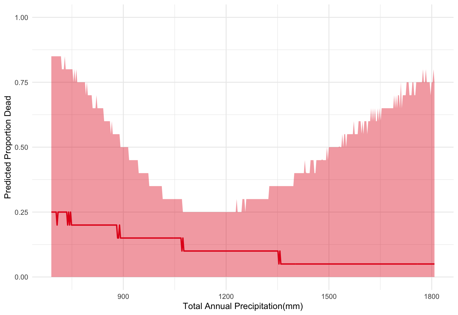
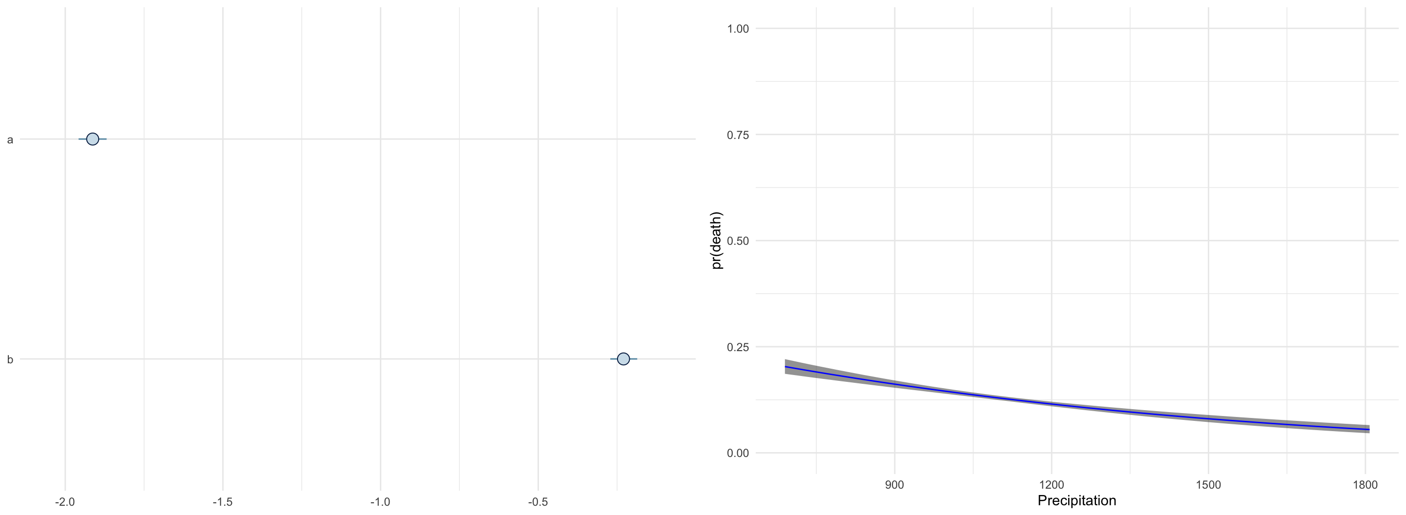
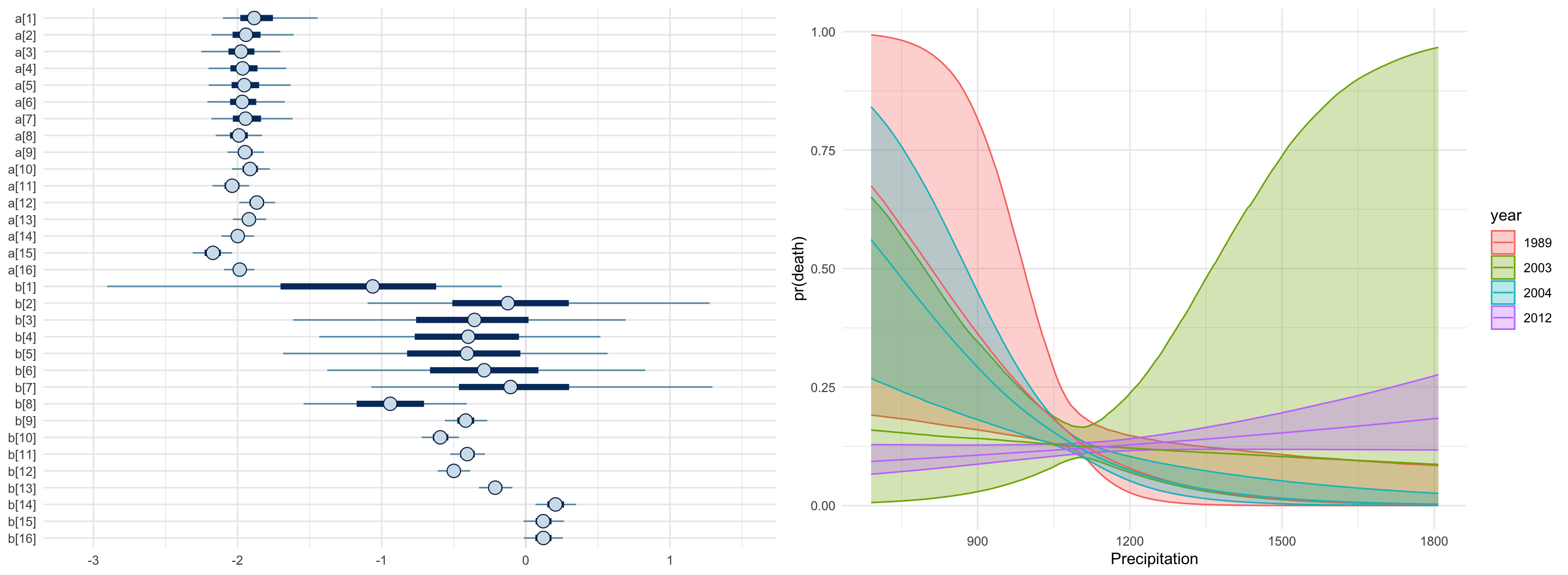
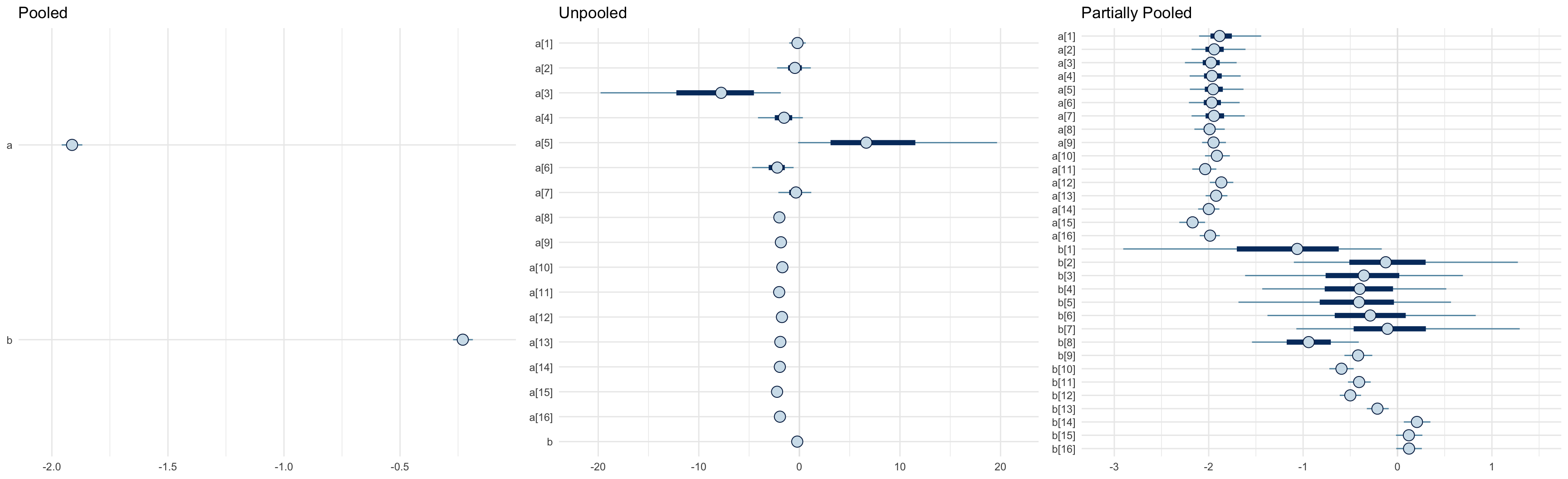
newx = seq(min(standat$precip), max(standat$precip), length.out=400)
pars = data.frame(as.matrix(fit_ppool, pars=c("a_mu", "a_sig", "b_mu", "b_sig")))

# For our hypothetical, we need to decide how many trees we would see
# more trees means less sampling uncertainty
N = 20
sims = mapply(sim1, amu = pars$a_mu, asig = pars$a_sig,
              bmu = pars$b_mu, bsig = pars$b_sig, 
              MoreArgs = list(N = 20, precip = newx))
sim_quantiles = apply(sims, 1, quantile, c(0.5, 0.05, 0.95))

Hierarchical Models

Kidney cancer death rates in the US

Kidney cancer death rates in the US

Kidney cancer death rates in the US

Kidney cancer death rates in the US

Kidney cancer Stan model: global/constant rate

Kidney cancer Stan model: global/constant rate

Kidney cancer Stan model: global/constant rate

Kidney cancer Stan model: rates per county

Kidney cancer Stan model: partial pooling

Kidney cancer Stan model: partial pooling

Kidney cancer Stan model: partially pooled rates per county

Kidney cancer Stan model: partially pooled maps

Kidney cancer Stan model: partially pooled maps

Precipitation-mortality relationships in Tsuga

Precipitation-mortality relationships in Tsuga: H1

Precipitation-mortality relationships in Tsuga: H2

Precipitation-mortality relationships in Tsuga: H3

Pooled model: code

Pooled models trade accuracy for precision

Pooled models trade accuracy for precision

Unpooled model: code

Unpooled model: code

Unpooled models use less data per parameter

Unpooled models use less data per parameter

Compromise: partial pooling

Partial Pooling: Code

Partial pooling is a compromise

Partial pooling is a compromise

Pooling comparison

Pooling comparison

When do we need hierarchical models?

When do we need hierarchical models?

When do we need hierarchical models?

Designing hierarchical models in Stan

Designing hierarchical models in Stan

Designing hierarchical models in Stan

Posterior predictive distributions

Posterior predictive distributions