There is no right solution to evaluation

Important to assess modelling goals before comparing models.

So why do we fit models?

Fit to calibration data
Predictive performance (new data)
Hypothesis testing
Avoiding overfitting

Rule of thumb: out-of-sample performance is the gold standard!

We can always improve fit to training/in-sample data by adding variables to the model

Information content & deviance

Entropy: how “predictable” is a distribution
High entropy means knowing the distribution tells us little about future observations
A useful metric is the average log probability
For \(n\) possible events, each with probability \(p_i\):

\[ H = -\mathbb{E}\left [\log \left (p \right) \right ] = -\sum_{i=1}^n p_i\log(p_i) \]

Entropy

Imagine a series of flips of a weighted coin:

pr_unfair = c(0.8, 0.2)
flips = sample(c("Heads", "Tails"), size = 20, replace = TRUE, prob = pr_unfair)
table(flips)
## flips
## Heads Tails 
##    17     3

A fair coin has high entropy; each face has a probability of \(\frac{1}{2}\), this (or any) sequence cannot help us predict the next roll

pr_fair = rep(1/2, 2)
-sum(pr_fair * log(pr_fair))
## [1] 0.6931472

An unfair coin has lower entropy; if we know which face is weighted, we can predict easily what the next outcome will be.

-sum(pr_unfair * log(pr_unfair))
## [1] 0.5004024

Principle of maximum entropy

The best model in a set is the one that maximizes the entropy of the residuals

After applying the model, the value of the residuals should tell us as little as possible about the next residual

Divergence

What’s the cost (how wrong will we be) of using the wrong model \(q\), when the true model is \(p\)
Or:
- How much extra entropy do we introduce by using model \(q\)?
This is known as the Kullback-Leibler (or K-L) divergence.

\[ D_{KL} = \sum_{i=1}^n p_i\log \left (\frac{p_i}{q_i} \right) \]

sum(pr_unfair * log(pr_unfair/pr_fair))
## [1] 0.1927448

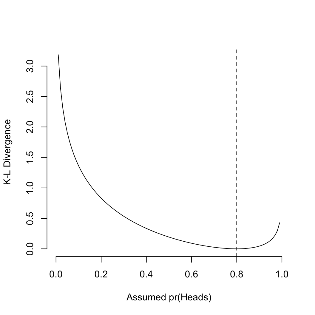
This tells us how much entropy we get from assuming our unfair coin is fair. This is a bad model: the prob of heads is really 0.8, but we assumed it was \(\frac{1}{2}\).

If the model is even worse, divergence increases. What if we assume \(pr(Heads) = \frac{1}{10}\) instead of \(\frac{1}{2}\)?

pr_10 = c(1/10, 1 - 1/10)
sum(pr_unfair * log(pr_unfair/pr_10))
## [1] 1.362738

The “true” model is unknown

We never have access to the true model \(p\) from this equation

\[ D_{KL} = \sum_{i=1}^n p_i\log \left (\frac{p_i}{q_i} \right) \]

We suspect our coin is weighted from the flips, but we don’t know the probs
Instead we estimate them by performing an experiment (flipping the coin) and building a model
We have two competing hypotheses: call them \(\theta_{map}\) and \(\theta_{fair}\)

\[ \begin{aligned} D_{KL, \theta_{map}} & = \sum_{i=1}^n \theta_{true}\log \frac{\theta_{true}}{\theta_{map}} \\ D_{KL, \theta_{fair}} & = \sum_{i=1}^n \theta_{true}\log \frac{\theta_{true}}{\theta_{fair}} \\ \end{aligned} \]

\(\theta_{true}\) cancels!
We can compare the models’ relative performance without knowing anything about \(\theta_{true}\)

log_likelihood = function(probH, flips)
    sum(dbinom(sum(flips == "Heads"), length(flips), prob = probH, log=TRUE))

log_posterior = function(probH, flips) {
    # a priori we expect 50/50 heads and tails, and I give the prior a bit of weight because most coins are fair
    log_likelihood(probH, flips) + dbeta(probH, 15, 15, log=TRUE) 
}

map = optim(pr_fair[1], method="Brent", log_posterior, flips=flips, 
            control=list(fnscale=-1), lower=0, upper=1)

# mle with no prior, for comparison
mle = optim(pr_fair[1], method="Brent", log_likelihood, flips=flips, 
            control=list(fnscale=-1), lower=0, upper=1)

prs_map = c(map$par, 1-map$par)
prs_mle = c(mle$par, 1-mle$par)
round(rbind(
    observed = table(flips)/sum(table(flips)),
    map = prs_map,
    mle = prs_mle
), 2)
##          Heads Tails
## observed  0.85  0.15
## map       0.65  0.35
## mle       0.85  0.15

Deviance

We can compare the models’ relative performance without knowing anything about \(\theta_{true}\)
We just need to know the entropy of each model: \(H_{\theta} = -\mathbb{E}\left [\log pr \left(x | \theta \right) \right ]\)
Deviance is an estimate of the entropy of a model:

\[ D = -2 \sum \log pr \left(x | \theta \right) \]

This is simply twice the log liklihood

Dmap = -2 * log_likelihood(prs_map[1], flips)
Dfair = -2 * log_likelihood(pr_fair[1], flips)
Dmle = -2 * log_likelihood(prs_mle[1], flips)

round(c(map = Dmap,mle = Dmle, fair = Dfair), 3)
##    map    mle   fair 
##  7.016  2.831 13.648

The MAP estimate has lower deviance, meaning it will predict new observations better than the hypothesis that the coin is fair
The prior has a significant effect as well!

Information criteria

Take two models, \(\theta_1\) has one parameter, \(\theta_2\) has two
If the models are nested (\(\theta_1\) is a subset of \(\theta_2\))
\(D_1\) will always be greater than \(D_2\)
- This is due to the increased flexibility gained by adding parameters
Thus we need a way of estimating out-of-sample deviance
- How well do the models fit data that were not used for calibration
Information criteria approximate this by penalizing models for complexity

\[ \mathrm{AIC} = 2k - D\left [ \mathbb{E} \left (\theta \right ) \right ] \]

AIC for the Tsuga model

Last time, we had three varieties of models for the effect of precipitation on Tsuga mortality.
We add a fourth here, with partial pooling but only for intercepts
1. Completely pooled
2. Unpooled intercepts (one intercept per year)
3. Partially pooled intercepts & slopes (hierarchical model)
4. Partially pooled intercepts (hierarchical model)

AIC for the Tsuga model

Last time, we had three varieties of models for the effect of temperature on Tsuga mortality
1. Completely pooled
2. Unpooled intercepts (one intercept per year)
3. Partially pooled intercepts (hierarchical model)
We can estimate the MAP values for the parameters using rstan::optimizing
We just need to modify the Stan program to compute the log likelihood and the deviance

generated quantities {
    real deviance = 0;
    vector [n] loglik;
    for (i in 1:n) {
        loglik[i] = binomial_lpmf(died[i] | n_trees[i], p[i]);
        deviance += loglik[i];
    }
    deviance = -2 * deviance;
}

AIC for the Tsuga model

library(rstan)
map_up = optimizing(tsuga_unpooled, standat)
map_p = optimizing(tsuga_pooled, standat)
k1 = sum(grepl("^[a|b]", names(map_p$par)))  # 2 parameters
k2 = sum(grepl("^[a|b]", names(map_up$par)))  # 17 parameters
aic = c(2*k1 - map_up$par["deviance"], 2*k2 - map_p$par["deviance"])
res = rbind(aic, aic - min(aic)); rownames(res) = c("AIC", "delta"); colnames(res) = c("Pooled", "Unpooled")
res
##            Pooled  Unpooled
## AIC   -5840.80002 -5865.183
## delta    24.38348     0.000

AIC prefers the more complex model:
- Priors must be uninformative or totally overwhelmed by the data
- Posterior must be multivariate normal
- Sample size must be very large relative to the number of parameters (n > ~25*k)
Moreover, AIC not well-defined for the hierarchial model
- Parameters are not independent, so the model is less “complex” than the unpooled

Deviance information critereon

Bayesian models often have difficult-to-estimate numbers of parameters
We can instead use posterior samples to approximate model complexity
- How much to models differ from the “best” model, on average

\[ \begin{aligned} p_D & = \mathbb{E} \left[ D \left (\theta \right ) \right] - D\left [ \mathbb{E} \left (\theta \right ) \right ] \\ \mathrm{DIC} &= D\left [ \mathbb{E} \left (\theta \right ) \right ] + 2p_D \end{aligned} \]

fit_up = sampling(tsuga_unpooled, standat, iter=5000, refresh=0, chains=1)
fit_p = sampling(tsuga_pooled, standat, iter=5000, refresh=0, chains=1)
fit_pp = sampling(tsuga_ppool, standat, iter=5000, refresh=0, chains=1)
fit_ipp = sampling(tsuga_int_ppool, standat, iter=5000, refresh=0, chains=1)

## note for the hierarchical model, a MAP is hard to find,
## here we use the min deviance as a quick and dirty estimate
## a better estimate is to compute the mean of all parameters, then 
## compute the deviance with those values
pd = c(Pooled = mean(as.matrix(fit_p, pars="deviance")) - map_up$par["deviance"],
    Unpooled = mean(as.matrix(fit_up, pars="deviance")) - map_p$par["deviance"],
    Hierarchical = mean(as.matrix(fit_pp, pars="deviance")) - min(as.matrix(fit_pp, pars="deviance")),
    Hierarchical_intercept = mean(as.matrix(fit_ipp, pars="deviance")) - min(as.matrix(fit_ipp, pars="deviance")))
dic = 1*pd + c(map_up$par["deviance"], map_p$par["deviance"], min(as.matrix(fit_pp, pars="deviance")),
             min(as.matrix(fit_ipp, pars="deviance")))
dic = rbind(dic, dic - min(dic)); rownames(dic) = c("DIC", "delta")
dic
##       Pooled.deviance Unpooled.deviance Hierarchical Hierarchical_intercept
## DIC         5901.1422         5860.5243     5754.922              5872.5218
## delta        146.2202          105.6022        0.000               117.5998

Log predictive pointwise density

For real models, DIC has some problems
- assumes posterior is multivariate normal
- only assesses the “best” fit, doesn’t fully use the posterior
- these can strongly influence inference, as well will see
Instead of considering deviance of each model, we can consider the probability of each data point
- This is closely related (but more fine-grained) to the penalty applied for DIC
- Instead of averaging within models, we average for each point across \(S\) posterior samples

\[ \mathrm{lppd} = \sum_{i=1}^n \log \frac{1}{S} \sum_{j=1}^S pr(y_i | \theta_j) \]

Cross validation

To best understand model performance, we should compare out-of-sample
Holdout/validation dataset
- separate, independent dataset not used for calibration
k-fold
- separate model into k “folds”
- For each fold, fit the model to all data not in fold
- validate against model in fold
- best model has best average performace across all folds
LOO
- For \(n\) data points, you fit \(n\) models
- Each time, you leave out one data point for validation

LOO

We can use the lppd to approximate LOO without the cost of fitting \(n\) models
Conceptually, AIC and DIC are attempts at approximating LOO
WAIC (Widely applicable information criterion) extends this, using lppd instead of deviance

LOO

We can use the lppd to approximate LOO without the cost of fitting \(n\) models
Conceptually, AIC and DIC are attempts at approximating LOO
WAIC (Widely applicable information criterion) extends this, using lppd instead of deviance
- It is pointwise, so it approximates the cost to model fitting of leaving out each point
- Averaged across the entire posterior

LOO

We can use the lppd to approximate LOO without the cost of fitting \(n\) models
Conceptually, AIC and DIC are attempts at approximating LOO
WAIC (Widely applicable information criterion) extends this, using lppd instead of deviance
- It is pointwise, so it approximates the cost to model fitting of leaving out each point
- Averaged across the entire posterior
Another technique, importance sampling, can directly approximate LOO
- These methods don’t always work, but when they doo, LOO/WAIC provide more robust estimates than DIC/AIC

LOO for trees

Package loo can estimate LOO-IC and WAIC for us. All that is needed is to compute the lpd (log pointwise density) in your Stan model.

generated quantities {
    vector [n] loglik; // vector, one per data point, because this is the pointwise density
    for (i in 1:n) {
        // here change binomial to whatever likelihood function applies to the model
        // lpmf: "log probability mass function"
        // for continuous distributions, use lpdf, e.g., normal_lpdf
        loglik[i] = binomial_lpmf(died[i] | n_trees[i], p[i]);
    }
}

LOO for trees

## put all models into a list for convenience when doing repeated operations
fits = list(unpooled=fit_up, pooled=fit_p, hierarchical=fit_pp, hierarchical_int=fit_ipp)

## get a loo object for each model
loos = lapply(fits, loo, pars="loglik")

loos$unpooled
## 
## Computed from 2500 by 1406 log-likelihood matrix.
## 
##          Estimate    SE
## elpd_loo  -2965.9 134.3
## p_loo        64.1   7.4
## looic      5931.8 268.5
## ------
## MCSE of elpd_loo is NA.
## MCSE and ESS estimates assume MCMC draws (r_eff in [0.4, 1.4]).
## 
## Pareto k diagnostic values:
##                          Count Pct.    Min. ESS
## (-Inf, 0.7]   (good)     1400  99.6%   74      
##    (0.7, 1]   (bad)         5   0.4%   <NA>    
##    (1, Inf)   (very bad)    1   0.1%   <NA>    
## See help('pareto-k-diagnostic') for details.

print(loo_compare(loos), simplify = FALSE)
##                  elpd_diff se_diff elpd_loo se_elpd_loo p_loo   se_p_loo
## hierarchical         0.0       0.0 -2917.0    132.9        76.1     8.8 
## pooled             -38.5      24.0 -2955.5    130.4         9.7     1.1 
## hierarchical_int   -43.6      21.8 -2960.7    133.3        48.1     5.2 
## unpooled           -48.9      23.0 -2965.9    134.3        64.1     7.4 
##                  looic   se_looic
## hierarchical      5834.0   265.9 
## pooled            5911.0   260.7 
## hierarchical_int  5921.3   266.5 
## unpooled          5931.8   268.5

Model weights

LOO/W/A/D IC can choose a “best” model for us
But all models are wrong, and even models that aren’t the best contain information
Akaike weights are a computationally simple way of performing mulimodel inference
- Roughly speaking, \(w_i\) is the probability that model \(i\) is the best model in the set of \(m\) models
- if using loo’s elpd_diff, can omit the \(-\frac{1}{2}\)

\[ w_i = \frac{e^{-\frac{1}{2}\Delta \mathrm{*IC}_i}} {\sum_{j=1}^m e^{-\frac{1}{2}\Delta \mathrm{*IC}_j}} \]

looics = sapply(loos, function(x) x$estimates['looic', 'Estimate'])
delta_looic = looics - min(looics)
wi = exp(-0.5*delta_looic) / sum(exp(-0.5*delta_looic))
round(rbind(looic = looics, dlooic = delta_looic, weight = wi), 2)
##        unpooled  pooled hierarchical hierarchical_int
## looic   5931.85 5910.96      5834.02          5921.32
## dlooic    97.83   76.94         0.00            87.29
## weight     0.00    0.00         1.00             0.00

Weights for multimodel inference

Akaike weights can help us decide how much to trust a single ‘best’ model
They underestimate information contained in the posteriors of the worse models
A more Bayesian approach is to make predictions, averaging the uncertainty from all models
For this we use stacking weights, which choose weights based on maximising the elpd from LOO

wts = loo_model_weights(loos)
wts
## Method: stacking
## ------
##                  weight
## unpooled         0.157 
## pooled           0.243 
## hierarchical     0.600 
## hierarchical_int 0.000

Bayesian model averaging

We can produce a posterior predictive distribution in Stan

generated quantities {
    vector [n] loglik; // vector, one per data point, because this is the pointwise density
    int ppd_died [n]; // predicted number of trees dying at each point in the original dataset
    for (i in 1:n) {
        // here change binomial to whatever likelihood function applies to the model
        // lpmf: "log probability mass function"
        // for continuous distributions, use lpdf, e.g., normal_lpdf
        loglik[i] = binomial_lpmf(died[i] | n_trees[i], p[i]);
        ppd_died[i] = binomial_rng(10, p[i]); // here I give a ppd assuming a sample size of 10 trees
    }
}

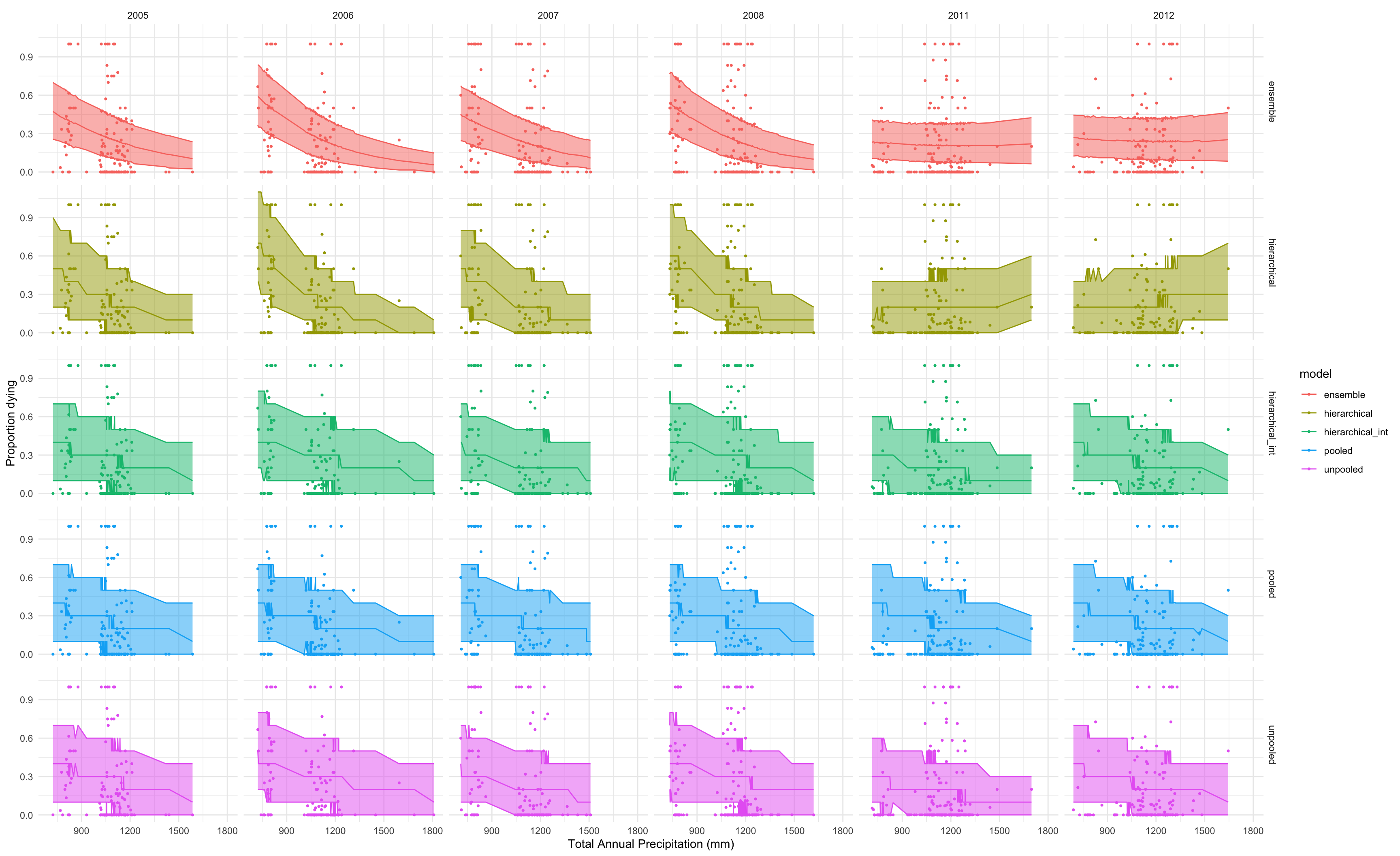
Then apply the weights to our predictions

ppd = lapply(fits, as.matrix, pars="ppd_died")
weighted_ppd = Map(`*`, ppd, wts)
avg_predictions = Reduce(`+`, weighted_ppd)

## now get some quantile intervals, put them alongside the original values and the temperature
quants = lapply(ppd, function(x) cbind(data.table(t(apply(x, 2, quantile, c(0.5, 0.05, 0.95)))), tsuga))
quants$ensemble = cbind(data.table(t(apply(avg_predictions, 2, quantile, c(0.5, 0.05, 0.95)))), tsuga)
quants = rbindlist(quants, idcol="model")
colnames(quants)[2:4] = c("median", "lower", "upper")

pl = ggplot(quants[year %in% c(2005:2008, 2011:2012)], aes(x=tot_annual_pp, y = median/10, colour = model)) + 
    geom_line() + 
    geom_ribbon(aes(x=tot_annual_pp, ymin= lower/10, ymax=upper/10, fill = model), alpha = 0.5, show.legend = FALSE) + 
    facet_grid(model ~ year) + theme_minimal() + geom_point(aes(x=tot_annual_pp, y = died/n), size=0.6) + 
    xlab("Total Annual Precipitation (mm)") + ylab("Proportion dying")

Model Selection & Comparison

There is no right solution to evaluation

There is no right solution to evaluation

Information content & deviance

Entropy

Principle of maximum entropy

Divergence

The “true” model is unknown

Deviance

Information criteria

AIC for the Tsuga model

AIC for the Tsuga model

AIC for the Tsuga model

Deviance information critereon

Log predictive pointwise density

Cross validation

LOO

LOO

LOO

LOO for trees

LOO for trees

Model weights

Weights for multimodel inference

Bayesian model averaging

Bayesian model averaging results